
Exploring the potential of battery electric buses for urban electricity peak load shaving
Pengshun Li, Kaisan Li, Jiayu Wang, Xiaoru Chen, Pengyuan Shen, He Qi, Yi Zhang
2026
eTransportation
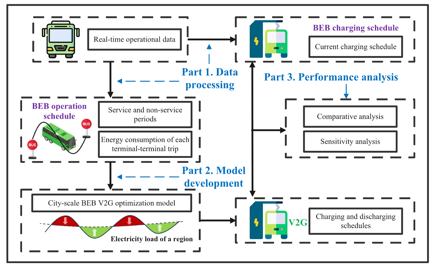
Fig. 1. Overview of the study.
Summary
This paper constructs a city-scale V2G optimization model based on real operational data of Shenzhen’s battery electric buses to evaluate grid peak-shaving potential. Compared with charging-only scheduling, bidirectional V2G operation reduces the peak-valley difference ratio by 35.4%–37.5%. Sensitivity analysis proves buses with over 60% non-service time perform best, and expanding fleet size works better than boosting charging power. V2G also improves the economic profit of bus fleets, providing practical urban energy management references.
Abstract
The adoption of vehicle-to-grid (V2G) technology, enabling the integration of electric vehicles (EVs) with the power grid, holds substantial potential for enhancing energy management. Battery electric buses (BEBs) are a key subset of EVs, and exploring their role in V2G offers an additional pathway for urban load shifting and improving grid flexibility. This study develops a city-scale BEB V2G optimization model to quantify the citywide peak-shaving potential of BEBs using real-world operational data from Shenzhen, China. Electricity demand over a week-long horizon is optimized by coordinating BEB charging and discharging at a 5-minute temporal resolution. Results show that charging-only optimization applied to 15,000 sampled BEBs, nearly the entire Shenzhen BEB fleet, reduces the average peak–valley difference ratio ( ) by 13.5% during a high-load week and by 14.5% during a low-load week. Under V2G participation, these reductions increase to 35.4% and 37.5%, indicating that discharging activities are essential for substantial peak-shaving gains. From an economic perspective, V2G service also improves profit. Each additional 1000 BEBs in V2G reduces by approximately 0.010, indicating strong scalability. Sensitivity analysis further shows that increasing charging/discharging power is effective when only a small number of BEBs engage in V2G; however, when more than 10,000 BEBs are available, further increases offer negligible additional benefit. Comparison across non-service time ratios reveals that BEBs with ratios below 40% contribute minimally to peak shaving, whereas those above 60% provide significantly greater reductions in . These findings suggest that BEBs with extended non-service periods should be prioritized for V2G participation.
1. Introduction
China’s commitment to reach carbon peak before 2030 and achieve carbon neutrality before 2060 has accelerated the adoption of electric equipment across multiple sectors [1]. While this transition reduces fossil fuel dependence, the widespread use of electric equipment also increases pressure on urban distribution grids. Uncoordinated electricity demand can amplify peak loads, degrade power quality, and reduce operational efficiency [2]. These challenges create an urgent need for effective load-shifting strategies to stabilize voltage levels and improve overall grid performance.
Traditional approaches to this challenge involve constructing peak ing power plants and constructing energy storage systems (ESS). Peak ing power plants are facilities that are designed to operate during short periods of high demand and remain idle for most of the year. However, they require high operating costs and often rely on fossil fuels, making them environmentally harmful [3]. ESS offers an alternative by storing electricity during low-load periods and releasing it during peak hours [4,5]. Yet, their deployment is capital-intensive, spacedemanding, and subject to strict safety requirements, which limits their scalability in urban grids.
In parallel with carbon neutrality efforts, China’s transportation system is undergoing rapid electrification [6]. By the end of 2023, there were 15.52 million EVs in China [7], and it is estimated that China’s EV penetration rate will reach 42.40% in 2030 and 52.97% in 2035 [8]. Shenzhen is a leading example of this transition. The city has electrified both private vehicles and public transportation, and in 2017 replaced more than 15,000 diesel buses with battery electric buses (BEBs), forming the largest BEB fleet in the world [9]. These electrified fleets create large onboard battery resources with controllable safety management systems and standardized recycling solutions.
Vehicle-to-grid (V2G) technology provides a way to utilize these distributed batteries for urban load shifting. V2G enables bidirectional energy exchange between vehicles and the grid. Vehicles discharge energy during high-load periods to reduce peak demand and recharge during low-load periods to fill load valleys. Previous studies have shown that V2G participation by private electric vehicles can reduce local peak loads and improve load profiles, revealing the potential of using mobile batteries as flexible energy buffers [10–12]. However, private EV owners face multiple barriers that limit large-scale V2G adoption, including limited financial incentives and challenges in coordinating individual participation [13]. These challenges reduce the reliability and effectiveness of V2G when relying solely on private vehicles. In contrast, BEB fleets offer a unique opportunity. BEBs operate on fixed schedules, follow predictable routes, and charge at central ized depots equipped with standardized management systems. These characteristics simplify coordination and eliminate many uncertainties associated with private EV V2G participation.
Despite these advantages, no existing study has quantified the system-level potential of using BEBs for V2G in citywide peak shaving. This gap is notable because BEB fleets represent substantial, control lable, and highly predictable energy storage resources in many rapidly electrifying cities. Understanding whether BEBs can meaningfully contribute to citywide peak shaving, and whether V2G participation is necessary beyond charging optimization, can inform energy planning, enhance grid flexibility, and support long-term carbon neutrality goals.
To achieve this, this study explores the potential of utilizing BEBs in V2G for peak shaving using real-world BEB operation data. The main contributions of this study are as follows:
• A city-scale BEB V2G optimization model, designed to minimize city load variance, has been developed to assess the potential of BEBs for providing V2G services. Using real-world BEB operational data from Shenzhen, the model optimizes electricity demand over a week-long horizon by coordinating BEB charging and discharging at a 5-minute temporal resolution;
• Comparative analyses of charging-only optimization and V2G optimization against original charging schedules have been conducted to evaluate the impacts of BEB participation in V2G;
• Sensitivity analyses on the number of BEBs in V2G, charging/discharging power levels, and non-service time ratios have been conducted to further examine system scalability and operational robustness.
The remainder of the paper is organized as follows. Section 2 reviews the existing literature on load-shifting strategies. Section 3 presents the framework for evaluating the potential of utilizing BEBs in V2G for peak shaving. Section 4 describes the study area and the collected BEB data. Section 5 presents the results of the optimized BEB charging and discharging schedules and conducts comparative and sensitivity analyses. Finally, the conclusions are presented in Section 6.
2. Literature review
There are three main approaches to address uncoordinated electricity demand: constructing peaking power plants, constructing energy storage systems, and utilizing V2G technology. Both peaking power plants and ESS are stationary, infrastructure-intensive resources that provide peak-shaving through centralized operation. In contrast, V2G leverages mobile and distributed onboard batteries, offering flexible and scalable load-shifting capabilities without additional construction. This section reviews the existing studies on these approaches.
2.1. Peaking power plants and energy storage systems
Peaking power plants have historically played an important role in supporting power system reliability. These units provide fast-ramping and dispatchable capacity that can respond within minutes to sudden increases in electricity demand. Because of this capability, they are effective for covering short-duration peaks and stabilizing the grid during periods of high load or variable renewable generation [14,15]. However, they typically operate with very low-capacity factors and remain idle for most of the year. Despite this limited use, they incur high operating costs and rely heavily on fossil fuels, which leads to significant greenhouse gas emissions and environmental impacts [3]. These drawbacks reduce their suitability in modern power systems that are moving toward deep decarbonization and higher shares of variable renewable energy. As renewable penetration increases, the need for flexible and clean peak-shaving resources becomes even more pressing.
Therefore, industry and researchers began to research the possibility of replacing peaking power plants with energy storage system (ESS). ESS can charge during low-load periods and discharge during peak hours, which reduces dependence on peaking units [4]. They offer a cleaner way to manage load fluctuations. Some researchers analyzed the necessity, social equity, and costs of replacing peaking power plants with ESSs [16–18]. Other researchers explore the suitable capacity and locations of ESS. For example, [19] developed an optimization model to optimally determine the size and site of an ESS connected to a distribution network for peak shaving and reliability improvement under system normal and outage scenarios. Similarly, [20] built a frequency response model based on emergency frequency regulation to configure the energy storage capacity. In addition, some studies are on the quantification of benefits of utilizing ESS. For example, [21] found that integrating an ESS into a fast-charging station significantly reduces peak power loads from the station by 19.01%–22.68%. Similar findings were reported by [22], where ESS installation reduced peak operating power by 41%. Moreover, the research conducted by [23] indicated that with ESS, the energy cost is reduced by significant 6.9% and CO2 emissions is decreased by 8.6%.
Although ESS provides effective peak-shaving capabilities, its adoption is constrained by high investment costs, as documented in multiple studies and technical assessments [22,24]. For example, it was reported that the cost of installing an ESS in a fast-charging station reaches up to 27,408 RMB/day [22]. Additionally, large-scale battery installations require significant space and may raise safety concerns. These limitations have motivated growing interest in alternative flexible resources that can provide similar load-shifting benefits without the high upfron costs associated with stationary storage.
2.2. Vehicle-to-grid technology
V2G technology has emerged as a promising distributed solution for load shifting and supporting power system flexibility. Unlike stationary energy storage systems, V2G utilizes the aggregated battery capacity of including private electric taxis, and BEBs, to provide bidirectional power flow between vehicles and the grid. During periods of low electricity demand or high renewable generation, EVs can charge and store energy; during peak-load periods, they can discharge electricity back to the grid when they have sufficient state-of-charge [25–27]. This decentralized operational feature makes V2G an attractive complementary resource to traditional peaking power plants and stationary ESS.
A growing body of literature has evaluated the potential of V2G for peak shaving. Early studies demonstrated that even modest participation rates of EVs can substantially reduce system peak load due to the large number of mobile batteries distributed across urban area [28]. More recent research has incorporated high-fidelity travel behavior data, charging patterns, and fleet-level operational characteristics. For example, [11] developed a coupled mobility-V2G framework that captures individual private EV travel-charge behaviors. Applying the framework to 480,000 private EVs in Shenzhen, the study found that V2G could reduce the citywide peak–valley ratio by 73%. Similarly, [29] analyzed V2G flexibility in large-scale electric taxi fleets, showing that under a fleet of 19,900 taxis, V2G could provide at least 50 MW for 1 h, 30 MW for 2 h, and 20 MW for 3 h during peak periods.
However, as noted in Section 1, private EV owners face multiple barriers that limit large-scale V2G adoption. This challenge has led researchers to explore BEBs, which can be centrally managed and therefore offer more controllable participation. Several studies have examined electric school buses, which have long daily idle periods and thus are well suited for V2G pilot experiments. [30] evaluated 200 electric school buses and found that V2G participation reduced the peak-to-average load ratio by 9.5% and school electricity bills by 22.6%. Other studies have investigated small BEB fleets, such as 11 BEBs in a medium-sized Portuguese city [31], 18 BEBs in a mid-size Japanese city [32], or BEBs operating across 20 depots in Korea [33]. Yet, these studies are limited to localized or depot-level analyses. Citylevel evaluations of BEB-based V2G remain scarce, making it difficult to inform the design and implementation of practical V2G policies for urban public transit systems. Therefore, understanding whether BEBs can meaningfully contribute to citywide peak shaving, and whether V2G participation is necessary beyond charging optimization, can provide valuable insights for energy planning, enhance grid flexibility, and support long-term carbon neutrality goals.
3. Methodology
3.1. Overview
Fig. 1 provides an overview of the proposed methodology for utiliz ing BEBs in V2G for peak shaving. The study consists of three parts: (i) data processing, (ii) model development, and (iii) performance analysis.
For data processing, real-world real-time BEB data are collected and processed into two datasets: the BEB operational schedule and the BEB charging schedule. The service and non-service periods are represented in the BEB operational schedule, which includes energy consumption of each terminal-terminal trip and the available time slots for charging and discharging. The BEB operational schedule is then input into the developed city-scale BEB V2G optimization model to explore the peak-shaving potential of BEBs while ensuring that their operational schedules remain unaffected. Finally, comparative analyses are conducted among the current charging schedule, charging-only optimized schedules, and V2G optimized schedules, as well as across different bus operational schedules. Sensitivity analyses are further performed on the number of participating BEBs and the charging and discharging power levels.
3.2. City-scale BEB V2G optimization model
3.2.1. Objective
The goal of peak shaving is to reduce the variance of electricity load during a time period. Therefore, in this study, the objective function is to minimize the load variance, shown in Objective (1) and Constraint (2).
where C represents the index set of periods. M represents the index set of time slots, represents a subset of M, B represents the index set of BEBs, and represents the index set of terminal-terminal trips for BEB �. and denote the optimized electricity load at time slots � and respectively, while represents the original electricity load at time slot � after reducing the load of the current BEB charging schedule. and correspond to the maximum charging and discharging power of BEB respectively. and continuous variables with values ranging from 0 to 1, indicate the charging and discharging power coefficients at time slot � after completing the trip �. Therefore, and represent the actual charging power and discharging power.
In this study, the electricity load for a week-long period is optimized. The time slot interval is set to 5 min, resulting in 2016 time slots, . Given the differences in electricity load between weekdays and weekends, the variances for these two periods are calculated separately, and their average is used as the optimization objective. Thus, there are two periods, i.e., , where 0 represents weekdays and 1 represents weekends. It should be noted that and represent the power sent to and received from the grid. Due to energy losses during transmission, the actual charging power for BEBs is slightly lower than , while the discharging power is slightly higher than . The charging and discharging efficiencies are reflected in the following section. Additionally, it is worth mentioning that the original electricity load may be different with different number of BEBs participating in V2G, as the electricity load caused by these BEB charging schedules are reduced.
3.2.2. Charging and discharging time constraints
Constraints for charging and discharging times are shown in Constraints (3a)–(4b):
where and represent the departure time and travel time of trip � for BEB and and represent the start and end times of time slot �. Constraints ensure that charging or discharging can only occur after BEB � completes trip �, while Constraints (4a)–(4b) ensure that charging or discharging must end before the successive trip � + 1.
3.2.3. Battery constraints
Constraints for battery are shown in Constraints :

Fig. 1. Overview of the study.
(11)
where represents the battery remaining energy (kWh) at the start of trip � for BEB and is the consumed energy (kWh) of trip � for BEB �. represents the charging or discharging amount at time slot � for BEB � after completing trip �. ��(�) and represent the first available time slot and last available time slot for charging or discharging activities after completing trip respectively. and represent the charging and discharging efficiency. represents the lower bound of . Constraints (5)–(6) track the battery energy changes between two consecutive trips. Constraints (7)–(8) ensure that the battery energy does not exceed the prescribed maximum requirement and remains above the minimum requirement for the following trip. Constraints (9)–(10) ensure that the battery energy does not exceed the battery capacity and remains nonnegative during the interval between two consecutive trips. Constraint (11) calculates the charging amount or discharging amount at each time slot.
3.2.4. Charging and discharging constraints
Charging and discharging cannot occur simultaneously, and this is shown in Constraints (14)–(16):
With Constraint (14). the optimization model becomes non-convex. resulting in slower and more complex solving process. There are numer ous studies on convex relaxation of this model, and the most common method is to add a penalty term in the objective function to avoid the simultaneous charging and discharging [34–38]. More specifically, the obiective function is reformulated as follows:
min
(18)
where captures the power loss during transmission and is a penalty coefficient with an arbitrary small value. This penalty term physically represents the reduction of transmission times to save energy. Therefore, the objective function considers both peak shaving and energy saving. With this penalty term, simultaneous charging and discharging can be avoided, i.e. and the model become a convex optimization model, which can be solved faster. The proof is given in Appendix. Besides, the result in the case study also validates the effectiveness of using this penalty term. After reformulation, Constraints (2)–(13) and (15)–(18) constitute the city-scale BEB V2G optimization model.
3.3. Peak-shaving performance measurement
The objective function in Section 3.2.1 minimizes the load vari ance over the optimization horizon, which serves as a continuous and tractable proxy for peak-shaving. To comprehensively evaluate peakshaving performance from different perspectives, multiple performance indicators are adopted. These indicators include the average daily peak–valley difference ratio , the average daily load flatness index (���), and the average daily standard deviation of load (���). Specifically, ��� is directly related to the optimization objective. In contrast, ���� and ��� are dimensionless indicators that normalize peak–valley differences and load flatness, respectively. These dimensionless metrics enable fair comparison across different scenarios and system scales, and provide additional operational insights that are not captured by variance alone. Together, these metrics offer complementary and consistent evaluations of how the variance-based optimization objective translates into practical peak-shaving benefits. The formulas of these three indicators are shown as follows:

(a) A representative week in March with low citywide electricity load

(b) A representative week in July with high citywide electricity load
Fig. 2. The electricity load of Shenzhen in two representative weeks.
where � represents the total days in the optimization range, and represent the maximum load and minimum load during the day respectively. is a vector recording the load during the day � and denotes the standard deviation of load at the day �.
4. Study area and data collection
4.1. Study area
Shenzhen is a major sub-provincial city on the central coast of southern Guangdong province and is a leading global technology hub often referred to as the ‘‘next Silicon Valley’’. Spanning 1952.84 square kilometers across nine districts, the city had a population of 17.66 million in 2023. Its gross domestic product (GDP) reached 3460.6 billion RMB (approximately 372.27 billion USD), ranking third among all Chinese cities.
With its large population and thriving manufacturing and technology sectors, Shenzhen exhibits substantial electricity demand across residential, commercial, and industrial sectors. The highest load, reaching approximately 20,000 MW, occurs in July when temperatures exceed During this period, air conditioning systems and refrigeration units consume a significant amount of electricity to maintain comfortable indoor temperatures and preserve perishable goods. In contrast, the lowest loads occur in March when the temperatures are around , with the maximum load of 12,500 MW. Fig. 2 shows the representative electricity load of the whole city for a low-load week in March and a high-load week in July. These two boundary scenarios enable us to evaluate the potential of utilizing BEBs for peak shaving through V2G under both mild and highly stressed grid conditions.
Additionally, Shenzhen has been strongly committed to green transportation and reducing emissions from public transit. Since 2017, the city has fully transitioned to a BEB fleet, replacing all fossil fuelpowered buses with more than 15,000 BEBs operating across over 900 bus lines, making it the largest BEB fleet in the world. Fig. 3 shows the locations of 951 bus lines and depots in Shenzhen, obtained from Amap (https://www.amap.com/). Depots are equipped with charging facilities, and BEBs return to these depots for charging during their non-service periods. In this study, we assume that all depots will be equipped with V2G technology, allowing BEBs to transmit energy to the power grid when they have sufficient power. This assumption is made deliberately. The goal is to evaluate the upper bound of the potential contribution of BEBs to citywide peak shaving. Therefore, we focus on the theoretical maximum V2G potential at the system level rather than the current technical or operational constraints of the power grid. By estimating this upper bound, the analysis provides decision-makers with a clear understanding of the maximum achievable benefits, which can inform further investigations into the practical deployment of V2G infrastructure in Shenzhen.
4.2. BEB travel data processing
It is noted that each BEB was equipped with an on-board terminal to record travel data at a sampling frequency of 0.1 Hz when purchased. Each data entry records the bus ID, current time, vehicle status, charging status and current state-of-charge (SoC). These real-time data help quantify the potential of BEBs in peak shaving. Fig. 4(a) shows a slice of raw BEB travel data, recorded every 10 s. The data within the red rectangle represents the operational data during a service period, which were processed into a row recording the start and end times, as well as the consumed SoC during this service period in Fig. 4(b). The data within the green rectangle correspond to a non-service period. It is noted that during this non-service period, the BEB was charging, with its SoC increasing from 70% to 80%. The data were processed into a row recording the start and end times of the non-service period in Fig. 4(b). Additionally, the charging activity during this period was also processed as a row in Fig. 4(c), reflecting the current charging schedule. With the processed operational data, the energy consumption of all BEBs during each service period, as well as the available periods for charging and discharging, are known, which helps explore the potential of BEBs in participating in V2G.
Due to data availability, travel data from only 960 BEBs belonging to 100 bus lines, collected between March 18 and 24, were used in this study. These BEBs are BYD e-buses with a battery capacity of 324 kWh corresponding to 100% SoC. Fig. 5 compares the length distributions of all 951 bus lines in Shenzhen with those of the 100 lines in the dataset. The median and mean trip lengths of the 951 lines are 13.9 km and 16.8 km, respectively, whereas those of the 100 collected lines are 12.7 km and 15.8 km. The differences in both median and mean values are only about 1 km. Trip length is strongly correlated with departure headway in bus operations, as lines of similar length typically follow comparable operational schedules due to consistent traffic conditions and similar round-trip cycle times. This similarity in trip-length distributions therefore indicates that the 100 collected lines exhibit service patterns broadly representative of the full set of lines in Shenzhen. Combined with the fact that nearly all BEBs in Shenzhen are of the same vehicle type, the 960 BEBs included in this study can be considered reasonably representative of overall BEB operational behaviors. It is also important to note that this study aims to explore the potential of utilizing BEBs for V2G-based peak shaving, rather than to perform detailed charging-schedule optimization. Therefore, the analysis does not require the same level of scheduling precision as an operational optimization study would. However, if more detailed operational information from additional lines becomes available in the future, this component of the analysis can be further refined. To examine scenarios involving different numbers of participating BEBs, additional BEBs were randomly sampled from the 960 available BEBs. Because BEB operation schedules remain largely unchanged throughout the year, the schedules collected in March were also adopted for the July peak-shaving analysis.

Fig. 3. The locations of bus lines and depots in Shenzhen.
(a) Raw data

(b) Processed operational data
Fig. 4. An example of raw BEB travel data processing.

Fig. 5. Length distribution of 951 bus lines in Shenzhen and 100 bus lines from the collected data.
4.3. Current BEB charging analysis
After processing the raw BEB data, the current operational schedules are further investigated. Fig. 6 shows the number of BEBs out of service over time (out of a total of 960 collected BEBs) and the electricity load of Shenzhen during two representative weeks for comparison. In this study, a day is defined as starting at 4 a.m. and ending at 4 a.m. the next day. This is because the BEBs in Shenzhen start to operate after 4 a.m., and this setting facilitates the modeling of charging and discharging of BEBs. It is also noted that the minimum electricity loads every day also occur at around 4 a.m., but at that time, all BEBs are out of service. Therefore, this is a potential charging period for BEBs to fill the demand valley. Further, it is seen that fewest BEBs are available at 8 a.m.–10 a.m. and , as these periods are peak travel periods, and the bus service increases in frequency. The electricity loads during these periods are not relatively high. Therefore, for these periods, BEBs may not be much available to shave the demand peak. Additionally, there is a noticeable small spike in the available number of BEBs at the midday, while the electricity loads during this time reach the maximum over the whole day. Therefore, this is a potential discharging period for BEBs to shave the demand peak. This preliminary analysis proves the feasibility and potential of utilizing BEBs for shaving the electricity peak load of the city.
Fig. 7 shows the distribution of the proportion of non-service time in a week for these BEBs. The maximum non-service time ratio reaches 80%, indicating that this BEB operates for only 4.8 h per day. The minimum non-service time ratio is around 38%, indicating that thi BEB operates for approximately 15 h a day and has little time for rest. Additionally, the mean and median non-service time ratios are both around 59% (9.84 h a day). This also suggests that most BEBs have sufficient non-service time and should be capable of contributing to peak shaving.
Fig. 8 shows the charging schedules of the sampled 15,000 BEBs. The number 15,000 can be regarded as the approximate total number of buses operating in Shenzhen [9]. This figure illustrates the electricity load with and without BEB charging, where the area between the two curves reflects the activities of the current charging schedules. It can be observed that BEBs primarily charge during late-night hours and occasionally during midday. However, the charging does not occur strictly during the lowest-demand period of the day (around 4 a.m.). Shifting the existing charging demand toward deeper load valleys would help reduce the peak–valley difference. Additionally, since the electricity load during midday is already very high, BEB charging during this period further increases the pressure on the grid. These observations indicate that the current charging schedules have the potential to be improved to reduce the peak–valley difference in the overall city load. On the other hand, the present BEB charging demand accounts for only a small portion of the overall electricity load, meaning that BEBs themselves are not the dominant consumers of electricity. Instead, their significance lies in their role as mobile energy-storage carriers. This characteristic opens opportunities to explore whether BEBs could discharge electricity back to the grid during their non-service periods to shave peak demand. The combination of flexible charging windows and large aggregated battery capacity therefore provides a promising foundation for studying the potential of V2G strategies.
5. Results and discussion
5.1. Optimization model parameters and computational performance
Based on the collected historical BEB charging data, the maximum charging power is set to 155 kW in this study. Similarly, we assume that the maximum discharging power equals the charging power, also set to 155 kW. The charging efficiency and discharging efficiency are set to 0.9 and 0.95, respectively. Additionally, the maximum battery energy is set to 324 kWh, corresponding to 100% SoC. The initial battery energy for each BEB � is set to the value collected from real data at the start of the test week, and the final energy must be greater than or equal to this initial value. Furthermore, considering range anxiety and battery health, is set to the energy consumption of trip � plus 32.4 kWh (10% SoC). The reason for using kWh instead of SoC as the unit is that different BEBs have varying battery capacities, and kWh provides a standardized measurement, although in this study, all BEBs are identical.
Additionally, the optimized results and computational times of the original non-convex model and the convex relaxation model are compared, as shown in Table 1. The optimization is performed using Gurobi on a PC with the following specifications: Intel Core i9 processor (3.00 GHz, 24 cores) and 64 GB of RAM. It is noted that the penalty coefficient � is set as small as possible while ensuring that the simultaneous charging and discharging do not occur. After testing different values, � is set to 0.004 in this study. It is observed that when the optimization model includes only 960 BEBs, the optimized result is obtained in 7.57 h. However, when the model includes 5000 BEBs, the optimized result cannot be obtained within 72 h. In contrast, converting the model into a convex relaxation form significantly speeds up the solution. The model with 960 BEBs is solved in just 36 s, making it 750 times faster. Additionally, the obtained � value is only 0.32% worse than the exact solution. Furthermore, simultaneous charging and discharging are not observed in the solution of the convex relaxation model. This indicates that the convex relaxation model not only speeds up the solution but also produces result very close to the exact solution.

Fig. 6. The number of available BEBs versus electricity load over time.

Fig. 7. Distributions of non-service time for BEBs.
Table 1
Comparison between the original non-convex model and the convex relaxation model.

Fig. 8. The current BEB charging schedule and its impact on the electricity load.

Fig. 9. Citywide electricity loads after charging-only optimization and V2G optimization for 15,000 sampled BEBs.
5.2. Comparison between charging-only optimization and V2G optimization
Firstly, it is important to determine whether using BEBs for V2G i necessary or whether adjusting their charging schedules alone is sufficient for peaking shaving. To examine this question, a comparison is conducted between charging-only optimization and V2G optimization. Charging-only optimization means that BEBs do not discharge; only their charging schedules are shifted. In the optimization model, this is implemented by setting to 0 for all time slots. In contrast, V2G optimization allows both charging and discharging, and the corresponding schedules are regenerated.
Fig. 9 shows the original citywide electricity load and the loads ob tained after applying charging-only optimization and V2G optimization for 15,000 sampled BEBs. The results indicate that the charging-only optimization cannot reduce the peak around 12 p.m., because BEBs are not the main contributors to the load at that time, as shown in Fig. 8. Instead, charging-only optimization shifts the original late-night charging behavior from 10 p.m.–3 a.m. to 2 a.m.–5 a.m., which raises the lowest load. As a result, the charging-only strategy reduces ���� by 13.5% in the week with the highest average load and by 14.5% in the week with the lowest average load.
In contrast, V2G optimization enables BEBs to discharge during high-load hours (10 a.m.-4 p.m.) and to charge more during low-load hours. This combination reduces the peak and further raises the lowest load. With V2G, ���� can be reduced by up to 35.4% and 37.5% in the two representative weeks. These results show that V2G provides much stronger peak-shaving benefits than adjusting charging schedules alone, when BEBs are allowed to participate in discharging.
5.3. Impact of the number of BEBs in V2G on citywide load peak shaving
In this section, the impact of different numbers of BEBs participating in V2G on city load peak-shaving is explored. Fig. 10(a) illustrates how the city load becomes smoother as more BEBs participate in V2G. It is observed that during 12 a.m.–4 a.m., when the load is at its lowest, it significantly increases due to more BEBs charging at that time. The lowest load increases by 16.7% with 15,000 BEBs participating in V2G. Similarly, during 10 a.m.–4 p.m., when the load is at its highest, it significantly decreases as more BEBs discharge. However, the peak-shaving effect is not as good as valley-filling, as the highest load decreases by 3.8% with 15,000 BEBs participating in V2G. This is because the number of BEBs out of service during peak city load hours is much smaller than during low-load hours, as shown in Fig. 6.
Additionally, it is found that the peak-shaving effect on weekends is much better than on weekdays. This is because the original peak valley difference at weekends is smaller, while the bus service frequency is slightly lower, giving BEBs more time to charge and discharge. Comparing the peaking shaving effects in two representative weeks, it is observed that, with the same number of BEBs participating in V2G, the peak-shaving effect is much better in the week with the lowest average load, as shown in Fig. 10(b). For instance, in the scenario with 15,000 BEBs in V2G, ���� decreases by 37.5% in March compared to

(a) Optimizing the city load with different numbers of BEBs participating in V2G

(b) the peak-shaving performance measurement

(c) the fitted relationship between PVDR and number of BEBs participating in V2G

Fig. 10. Peak-shaving performance with different numbers of BEBs participating in V2G.
35.3% in July, ��� increases by 28.2% compared to 21.5%, and ��� decreases by 31.2% compared to 25.0%.
Fig. 10(c) shows the fitted relationships between the number of BEBs participating in V2G and the mean and median daily PVDR values, quantifying the marginal impact of adding one BEB to V2G on the city load. For the week with the lowest average load, adding every 1000 BEBs decreases the mean and median daily PVDR by 0.010 and 0.011, respectively. For the week with the highest average load, the decreases are 0.0089 and 0.0091, respectively. This fitted relationship can be viewed as an approximation of the marginal peak-shaving contribution of each additional BEB.
Fig. 11 shows the original charging time distribution as well as the optimized charging and discharging time distributions, along with the number of BEBs involved in charging and discharging at each time point for the week in July. The similar result can be observed for the week in March. It is noted that, in the current charging schedule, a noticeable number of BEBs charge at midday, at which time they should instead discharge according to the optimization results. The reason for midday charging is that BEB drivers typically allow the BEBs to charge while resting, ensuring enough SoC for trips in the second half of the day. However, analysis shows that discharging at midday would still ensure sufficient SoC for the BEBs. Therefore, it is recommended that BEBs should not charge at midday; rather, they should discharge if participating in V2G or refrain from charging if not participating. Additionally, another observation is that the night charging time is shifted 1 h later in the optimization result. This is because the lowest city load every day occurs at around 4 a.m. Shifting the charging time can effectively increase the lowest city load. Furthermore, it is observed that the main discharging periods are around 6 a.m.–7 a.m., 10 a.m.–11 a.m., 1 p.m.–5 p.m., and 8 p.m.–11 p.m. The reason why few BEBs discharge between 11 a.m. and 1 p.m. is that the city load decreases during this period, as it is a rest time when electricity demand is not relatively high. Therefore, BEBs do not need to discharge during this period, but instead save energy for discharging during other periods of high city load.

Fig. 11. Number of BEBs in charging and discharging over time for the week in July.
Moreover, with more BEBs participating in V2G, the concentrated charging and discharging periods shorten. This is easy to understand, as discharging or charging from a few BEBs already makes the load of certain periods optimal. Therefore, as the total number of BEBs increases, a smaller proportion of them engage in charging or discharging during these periods, causing them to become non-concentrated charging or discharging periods. On the other hand, the shortening of concentrated charging and discharging periods indicates that the remaining concentrated periods require more BEBs to participate, as the load during these periods is not yet optimal.
Fig. 12 illustrates the average charging and discharging amounts per BEB per day for different numbers of BEBs participating in V2G. It is observed that the difference between the daily charging and daily discharging amounts per BEB remains constant at 187 kWh, indicating that the average daily energy consumption for operation is 187 kWh. Additionally, it is noted that as more BEBs participate in V2G, their average charging and discharging amounts decrease. This can be explained by the fact that certain periods require only a few BEBs to engage, which reduces the average charging and discharging amounts. This phenomenon indicates that as more BEBs participate in V2G, the charging and discharging frequencies will deduce significantly, which benefits battery health.
5.4. Impact of charging and discharging power on citywide load peak shaving
Recently, many cities have increased or are going to increase the maximum charging/discharging power levels to over 400 kW [39, 40]; therefore, it is necessary to assess the impact of higher charging/discharging power on city load peak shaving. Fig. 13 presents the average daily PVDR (����) for different charging/discharging power levels and numbers of BEBs. To explicitly illustrate their impact, the corresponding number of BEBs with a charging/discharging power of 155 kW is displayed in the cell of each combination, calculated based on the fitted formula shown in Fig. 10(c). It should be noted that the relationship between number of BEBs and ���� (denoted as in Fig. 10(c)) is assumed to be linear, which may not be entirely accurate. This formula is used here to provide a rough estimate of the impact of different charging/discharging power levels.
The result indicates that when the number of BEBs participating in V2G is low, adopting higher charging/discharging power can significantly reduce ����. For instance, when only 960 BEBs participate in V2G during the week of July, increasing the charging/discharging power from 155 kW to 400 kW is equivalent to having 2.70 times more BEBs with a charging/discharging power of 155 kW. In contrast, when 15,000 BEBs participate in V2G, increasing the charging/discharging power to 400 kW is only equivalent to having 1.08 times more BEBs. Therefore, this suggests that when only a few BEBs are available for V2G participation, increasing the charging/discharging power is an effective strategy for shaving city load peaks. However, if a large number of BEBs can participate, increasing the charging/discharging power becomes less critical, especially when the budget for upgrading V2G infrastructure is limited.

Scenarios
Fig. 12. Average charging and discharging amounts per BEB per day with different numbers of BEBs participating in V2G.

(a) PVDR for the week in March

(b) PVDR for the week in July
Fig. 13. ���� for different combinations of numbers of BEBs and charging/discharging power levels.
5.5. Analysis of different bus operational schedules on citywide load peak shaving
Fig. 7 shows that different BEBs have different operational sched ules, resulting in varying non-service time ratios. The non-service time ratio refers to the proportion of time a BEB is not in service during a week. It is imperative to quantify the impact of different non-service time ratios on peak-shaving, so that decision makers can identify which BEBs to prioritize for initial V2G pilot implementation based on their operational schedules. Therefore, a comparative experiment with six scenarios is conducted. The base case is the one used in the previous analysis, where 15,000 BEBs are uniformly sampled from the 960 BEBs with a charging/discharging power of 155 kW. Scenarios A-E involve uniformly sampling 15,000 BEBs from specific groups with non-service time ratios between 30%–40%, 40%–50%, 50%–60%, 60%–70%, and 70%–80%, respectively.
Fig. 14 presents the peak-shaving performance of BEBs with different non-service time ratios participating in V2G. The performance of all BEBs with a non-service time ratio between 30%–40% (Scenario A) is the worst, reducing ���� by only 7.0% and 4.7% for the weeks in March and July, respectively, compared to the original load. This indicates that each BEB contributes and in two weeks to the reduction of ����, which is a negligible contribution. This result is reasonable, as these BEBs have little non-service time and operate throughout the day. They can only help fill the demand valley at night. For these BEBs, it is suggested that they do not need to participate in discharging activities, but shift the charging time to around 4 a.m., if possible, as analyzed in Section 5.3. As the sampled BEBs have higher non-service time ratios, the peak-shaving perfor mance improves. BEBs with non-service time ratios between 40%–50%, 50%–60%, 60%–70%, and 70%–80% each contribute , and , respectively, to reducing ���� in March, while contributing , and , respectively, in July. It can also be observed that the base case performs better than Scenario C but slightly worse than Scenario D. This pattern is consistent with its average non-service time ratio of 59%, which lies between the 50%–60% and 60%–70% ranges, shown in Fig. 7. These results suggest that peak-shaving performance improves noticeably when the participating fleet is dominated by BEBs with nonservice time ratios in the 60%–70% range or higher, while fleets with ratios below 50% provide only limited benefits. BEBs with non-service time ratios above 70% perform the best, as they are typically backup buses for emergencies or peak-hour services. However, their numbers may be limited. Therefore, decision makers should first quantify how

• Base case: 15000 sampled BEBs with non-service time ratios between 30%-80% Scenario A: 15000 sampled BEBs with non-service time ratios between 30%-40% • Scenario B: 15000 sampled BEBs with non-service time ratios between 40%-50% • Scenario C: 15000 sampled BEBs with non-service time ratios between 50%-60% • Scenario D: 15000 sampled BEBs with non-service time ratios between 60%-70% • Scenario E: 15000 sampled BEBs with non-service time ratios between 70%-80%
Fig. 14. Peak-shaving performance of BEBs with different non-service time ratios participating in V2G.
many of these high non-service time BEBs exist and prioritize their participation in V2G, where feasible.
5.6. Economic viability
The economic viability should be regarded as one of the major considerations in determining whether electric buses can participate in V2G services [41]. If V2G operation leads to financial losses, transit agencies will have little incentive to adopt V2G service. The main cost components include: (1) additional investment or upgrade costs for V2G-capable chargers and related infrastructure; (2) battery degra dation costs attributable to cycling; and (3) electricity purchase cost. When V2G services are enabled, additional revenue can be generated from electricity selling. This study does not consider infrastructure investment costs, as they are typically one-time fixed costs and are outside the scope of the daily operational analysis.
5.6.1. Battery degradation modeling
For the estimation of battery degradation cost, the previous work conducted by [42,43], and [11] is referenced in this study. The depth of discharge (DoD) of BEB � at time slot � is denoted as where is the battery remaining energy at time slot � and can be calculated based on , and �������� is the battery capacity. Then the DoD-number of cycles curve can be fitted via measurement [43]:
where �( is the number of cycles. and are coefficient characterizing the relationship between number of cycles and the DoD. They are set to , an , respectively, following the recommendations in . The degradation costs of BEB � at time slot � with respect to DoD can be calculated as follows:
where is the degradation cost at time slot is the unit investment cost, set as 917.4 RMB (132 USD) per kWh [42].
5.6.2. Electricity purchase and selling modeling
The electricity purchase price in Shenzhen is obtained from the official tariff information provided by the China Southern Power Grid [44], while the electricity selling price is referenced from the pricing document released by the Guangdong Provincial Development and Reform Commission [45]. The electricity purchase and selling prices at each time are presented in Fig. 15(a).
5.6.3. Economic viability analysis
Fig. 15(b) presents the costs under the original, charging-only optimized, and V2G-optimized schedules. It can be observed that the original schedule incurs the highest electricity purchase cost, as BEBs are sometimes charged during periods when purchase prices are very high, which is confirmed in Fig. 11. However, its battery degradation cost is the lowest, as it does not undergo more cycling than the charging-only and V2G-optimized schedules. Overall, the daily total profit, excluding operational income such as fare revenue, is −85.46 RMB. In contrast, the charging-only optimized schedule significantly reduces electricity purchase costs by forcing BEBs to charge during lowload periods, which coincide with lower electricity prices. However, its degradation costs are slightly higher than that of the original schedule because it performs more frequent, short charging cycles to optimize the electricity load, which accelerates battery wear. Overall, its daily total profit is −50.66 RMB.
Compared to these, V2G services allow BEBs to sell electricity. The daily electricity purchase cost and selling revenue per BEB are 83.87 RMB and 110.05 RMB, respectively, resulting in a profit of 26.18 RMB from electricity transaction. It should be noted that V2G operations involve much more cycling, leading to a daily battery degradation cost per BEB of 38.73 RMB. Nevertheless, the daily total profit is the highest among the three schedules, amounting to −12.55 RMB, primarily due to the electricity profit. Therefore, from an economic perspective, V2G not only supports city-scale electricity peak shaving but also improves financial viability.

(a) Electricity purchase and selling prices over time.
(b) Costs under the original, charging-only optimized, and V2G-optimized schedules (July scenario).
Fig. 15. Electricity purchase and selling prices, along with the results of the economic viability analysis.
5.7. Policy recommendation
The analyses in Sections 5.2–5.6 yield several implications for the design and implementation of V2G strategies in cities for BEB fleets. These implications highlight the conditions under which V2G can provide substantial peak-shaving benefits and identify operational con figurations that maximize system-level performance.
• Prioritize BEBs with high non-service time ratios. The compara- tive analysis in Section 5.5 shows that peak-shaving performance increases as the participating fleet contains more BEBs with non service time ratios above 60%, and BEBs with ratios above 70% exhibit the strongest performance. This suggests that initial V2G deployments should prioritize BEBs with extended non-service periods, as they provide the largest flexibility for controlled charg ing and discharging, and they do not affect daily service. There fore, early-stage V2G plans should focus on identifying these vehicles and including them in pilot deployments.
• Increase the number of participating BEBs before upgrading power levels. Higher charging and discharging power are most helpful when only a small number of BEBs are available. Once participation reaches roughly 10,000–15,000 vehicles, the marginal benefit of raising charging/discharging power levels declines sharply. Adding more BEBs has a larger impact on peak shaving than installing higher-power chargers. Therefore, cities should first encourage more BEBs to participate in V2G before investing in major power upgrades.
• Adjust charging schedules by reducing midday charging, allowing midday discharging, and shifting nighttime charging toward the load valley. A noticeable share of BEBs charges at midday in the current charging schedules, even though this period coincides with high city load. Optimization results show that these BEBs can safely discharge at this time without violating the required state of charge for service. Reducing midday charging helps lower peak load and improves V2G performance. Cities can achieve this by updating depot charging rules and using automated scheduling tools to shift charging to other periods. Additionally, the lowest city load occurs around 4 a.m., yet existing charging behavior tends to peak slightly earlier. Shifting nighttime charging closer to 4 a.m. can raise the minimum load more effectively and improve load flattening. This timing adjustment requires only operational coordination rather than infrastructure investment, making it a low-cost but impactful intervention.
6. Conclusions
This study examines the potential of utilizing BEBs for V2G par ticipation to support city load peak shaving. A city-scale BEB V2G optimization model that minimizes load variance is developed and implemented at a 5-minute temporal resolution to assess this potential. Real-world BEB operational data in Shenzhen, China, are used for analysis. A comparative evaluation of the current charging schedule, charging-only optimization, and V2G optimization is conducted to quantify the effect of BEB participation in V2G. Sensitivity analyses on the number of participating BEBs, charging/discharging power, and non-service time ratios further explore how these factors influence city load variance.
The results show that charging-only optimization applied to the 15,000 sampled BEBs, the nearly entire Shenzhen BEB fleet, reduces ���� by 13.5% in a high-load week and by 14.5% in a low-load week. Under V2G participation, these reductions increase to 35.4% and 37.5%, indicating that engaging BEBs in discharging activities is essential for achieving substantial peak-shaving gains. From an economic perspective, V2G services also improve overall profit. It is also estimated that each additional 1000 BEBs participating in V2G reduces ���� by approximately 0.0089 in high-load weeks and 0.010 in low-load weeks. The analysis of charging/discharging power levels shows that higher power is beneficial when only a small number of BEBs participate. However, once participation exceeds 10,000 BEBs, the marginal improvement from higher power becomes limited. The comparison of non-service time ratios reveals that BEBs with ratios below 40% contribute very little to peak shaving. In contrast, BEBs with ratios above 60% provide noticeably stronger reductions in ����, and those above 70% perform the best. These findings suggest that
BEBs with extended non-service periods should be prioritized for V2G participation.
The methods proposed in our study can be applied to other cities, even without fine-grained BEB data. Bus companies maintain bus operation schedules, which provide service and non-service periods for each BEB. For energy consumption data of each terminal-terminal trip, researchers can leverage energy consumption prediction models from existing studies, such as [46–48]. Thus, even with lower-resolution data, the potential of utilizing BEBs in other cities can still be explored. Several limitations of this study should also be acknowledged. This work aims to explore the upper bound of the potential contribution of BEBs to citywide peak shaving. Therefore, it focuses on the theoretical maximum V2G potential at the system level, rather than explicitly modeling current technical or operational constraints of the power grid. For this reason, charging infrastructure constraints, such as the number of chargers at individual depots, are not modeled in the current formulation. Such constraints have been explicitly considered in recent studies, for example by [49], who incorporated charger availability and depot-level power limitations when evaluating V2G-enabled public transport depots. Future research will incorporate charging infrastructure and power system constraints to assess practically attainable V2G performance and to investigate station-level and city-scale impacts under realistic operational conditions
CRediT authorship contribution statement
Pengshun Li: Writing – original draft, Methodology, Formal analy sis, Data curation, Conceptualization. Kaisan Li: Methodology, Concep tualization. Jiayu Wang: Visualization, Data curation. Xiaoru Chen: Supervision, Resources, Methodology. Pengyuan Shen: Supervision, Methodology, Investigation. He Qi: Validation, Supervision. Yi Zhang: Writing – review & editing, Supervision, Resources, Funding acquisi tion, Conceptualization.
Declaration of competing interest
The authors declare that they have no known competing finan cial interests or personal relationships that could have appeared to influence the work reported in this paper.
Acknowledgments
This research was supported by Shenzhen Science and Technology Program KCXST20221021111608020, Research and Development Project of Ministry of Housing and Urban-Rural Development of the People’s Republic China (Grant No. 2022-K-121).
Appendix. Proof of non-simultaneous charging and discharging by introducing the penalty term
Let and denote two pairs of charging/discharging power coefficients.
In the charging scenario, they satisfy:
Suppose h � > d have and their transmission losses are:
Obviously, therefore, the model ensures that only charging activities are allowed and prohibit discharging when charging. The same conclusion can be obtained for discharging scenario, where charging is prohibited.
Data availability
Data will be made available on request.
References
[1] State Council. Carbon peaking and carbon neutrality: China’s plans and solutions. 2025, https://english.www.gov.cn/archive/whitepaper/202511/08/ content WS690ee812c6d00ca5f9a076cd.html. [Accessed 07 December 2025]
[2] Liu J, Wang H, Du Y, Lu Y, Wang Z. Multi-objective optimal peak load shaving strategy using coordinated scheduling of EVs and BESS with adoption of MORBHPSO. J Energy Storage 2023;64:107121.
[3] Hojjatinia Z, Mezher AM, Castillo-Guerra E, Cardenas-Barrera J, Saleh SM. Peak shaving impact on load forecasting: A strategy for mitigation. IEEE Access 2024.
[4] Mitali J, Dhinakaran S, Mohamad A. Energy storage systems: A review. Energy Storage Sav 2022;1(3):166–216.
[5] Elalfy DA, Gouda E, Kotb MF, Bureš V, Sedhom BE. Comprehensive review of energy storage systems technologies, objectives, challenges, and future trends. Energy Strat Rev 2024;54:101482.
[6] Chen L, Msigwa G, Yang M, Osman AI, Fawzy S, Rooney DW, Yap PS. Strategies to achieve a carbon neutral society: a review. Environ Chem Lett 2022;20(4):2277–310.
[7] Monika. China has 20.41 million new energy vehicles running on roads by end of 2023. 2024, https://autonews.gasgoo.com/m/70030708.html. [Accessed 28 March 2025].
[8] Liu B, Song C, Liang X, Lai M, Yu Z, Ji J. Regional differences in China’s electric vehicle sales forecasting: Under supply-demand policy scenarios. Energy Policy 2023:177:113554
[9] Zheng W. Top 10 electric bus China. 2025, https://www.sourcifychina.com electric-bus-China/. [Accessed 28 March 2025].
[10] Zheng Y, Shao Z, Jian L. The peak load shaving assessment of developing a user-oriented vehicle-to-grid scheme with multiple operation modes: The case study of shenzhen, China, Sustain Cities Soc 2021:67:102744
[11] Li K, Li X, Xiong Z, Tao S, Zhao G, Jiang Y, Qi H, Zhang Y. Unlocking vehicle-togrid potential of load shifting in China's megacities considering comprehensive real-world behaviors. Nat Commun 2025;16(1):10087.
[12] Li Y, Wang K, Xu C, Wu Y, Li L, Zheng Y, Yang S, Wang H, Ouyang M. The potentials of vehicle-grid integration on peak shaving of a community considering random behavior of aggregated vehicles. Next Energy 2025;7:100233.
[13] Ravi SS, Aziz M. Utilization of electric vehicles for vehicle-to-grid services: Progress and perspectives. Energies 2022;15(2):589.
[14] Siemens Energy. Peaker power plants overview. 2024, https://www.siemensenergy.com/global/en/home/products-services/product/peaker-plants.html. [Ac cessed 08 December 2025].
[15] GAO. Electricity: Information on peak demand power plants. 2024, https://www. gao.gov/assets/gao-24-106145.pdf. [Accessed 08 December 2025].
[16] Porzio J, Wolfson D, Auffhammer M, Scown CD. Private and external costs and benefits of replacing high-emitting peaker plants with batteries. Environ Sci Technol 2023;57(12):4992–5002.
[17] Vu K, Ntakou E, Schlegelmilch J, Muse LP, Fioravanti R. Energy equity: Making the case for peaker plant replacement with battery energy storage. In: 2022 IEEE electrical energy storage application and technologies conference. EESAT, IEEE; 2022, p. 1–5.
[18] Tarekegne B, Powell D, Oikonomou K, Jacroux E, O’Neil R. Analysis of energy justice and equity impacts from replacing peaker plants with energy storage. In: 2022 IEEE electrical energy storage application and technologies conference. EESAT. JEEE: 2022. p. 1-5
[19] Inaolaji A, Wu X, Roychowdhury R, Smith R. Optimal allocation of battery energy storage systems for peak shaving and reliability enhancement in distribution systems. J Energy Storage 2024:95:112305.
[20] Chen X, Nan D, Xiong X, Chen H, Ma W. Energy storage capacity configuration planning considering dual scenarios of peak shaving and emergency frequency regulation. Processes 2024;12(4):743.
[21] Chen H, Hu Z, Zhang H, Luo H. Coordinated charging and discharging strategies for plug-in electric bus fast charging station with energy storage system, JET Gener Transm Distrib 2018;12(9):2019–28.
[22] Ding X, Zhang W, Wei S, Wang Z. Optimization of an energy storage system for electric bus fast-charging station. Energies 2021;14(14):4143.
[23] Zahari NEM, Mokhlis H, Mubarak H, Mansor NN, Sulaima MF, Ramasamy AK, Zulkapli MF, Ja’Apar MAB, Jaafar M, Marsadek MB. Integrating solar PV, battery storage, and demand response for industrial peak shaving: a systematic review on strategy, challenges and case study in Malaysian food manufacturing. IEEE Access 2024:12:106832–56
[24] Luo X, Wang J, Dooner M, Clarke J. Overview of current development in electrical energy storage technologies and the application potential in power system operation. Appl Energy 2015;137:511–36.
[25] Gnann T, Klingler AL, Kühnbach M. The load shift potential of plug-in electric vehicles with different amounts of charging infrastructure. J Power Sources 2018;390:20–9.
[26] Barone G, Buonomano A, Forzano C, Giuzio GF, Palombo A. Increasing selfconsumption of renewable energy through the Building to Vehicle to Building approach applied to multiple users connected in a virtual micro-grid. Renew Energy 2020;159:1165–76.
[27] Abdelfattah W, Abdelhamid AS, Hasanien HM, Rashad BAE. Smart vehicle-to-grid integration strategy for enhancing distribution system performance and electric vehicle profitability. Energy 2024;302:131807
[28] Lund H, Kempton W. Integration of renewable energy into the transport and electricity sectors through V2G. Energy Policy 2008;36(9):3578–87.
[29] Yu Q, Wang Z, Song Y, Shen X, Zhang H. Potential and flexibility analysis of electric taxi fleets V2G system based on trajectory data and agent-based modeling. Appl Energy 2024;355:122323.
[30] Khwanrit R, Javaid S, Lim Y, Charoenlarpnopparut C, Tan Y. Optimal vehicle to-grid strategies for energy sharing management using electric school buses. Energies 2024;17(16):4182.
[31] Manzolli JA, Trovao JPF, Antunes CH. Electric bus coordinated charging strategy considering V2G and battery degradation. Energy 2022;254:124252.
[32] Fei F, Sun W, Iacobucci R, Schmöcker JD. Exploring the profitability of using electric bus fleets for transport and power grid services. Transp Res Part C: Emerg Technol 2023:149:104060.
[33] Son J, Im J, Kim D. Urban transit optimization: Efficient electric bus operations and vehicle-to-grid integration. Comput Ind Eng 2025:111169.
[34] Yang P, Nehorai A. Joint optimization of hybrid energy storage and generation capacity with renewable energy. IEEE Trans Smart Grid 2017;5(4):1566–74.
[35] Li Q, Vittal V. Non-iterative enhanced SDP relaxations for optimal scheduling of distributed energy storage in distribution systems. IEEE Trans Power Syst 2016;32(3):1721–32.
[36] Yang S, Gao HO, You F. Integrated optimization in operations control and systems design for carbon emission reduction in building electrification with distributed energy resources. Adv Appl Energy 2023;12:100144.
[37] Wang Q, Wu W, Lin C, Xu S, Wang S, Tian J. An exact relaxation method for complementarity constraints of energy storages in power grid optimization problems. Appl Energy 2024;371:123592.
[38] Zheng L, Zhou B, Chung CY, Li J, Cao Y, Zhao Y. Coordinated operation of multienergy systems with uncertainty couplings in electricity and carbon markets. IEEE Internet Things J 2024;11(14):24414–27.
[39] NEWS. Shenzhen surpasses 500 supercharging stations, outnumbering gas stations. 2024, https://www.newsgd.com/node_5c070fdd03/2e2e1c4028.shtml. [Accessed 20 March 2025].
[40] Carla. Tesla brings its V4 supercharger to China. 2025, https://www.electrive. com/2025/01/03/tesla-brings-its-v4-supercharger-to-china/. [Accessed 26 March 2025].
[41] Zheng Y, Shao Z, Shang Y, Jian L. Modeling the temporal and economic feasibility of electric vehicles providing vehicle-to-grid services in the electricity market under different charging scenarios. J Energy Storage 2023;68:107579.
[42] Le LB, et al. Building energy management and Electric Vehicle charging consid ering battery degradation and random vehicles’ arrivals and departures. J Energy Storage 2023;64:107141
[43] Xu B. Oudaloy A. Ulbig A. Andersson G. Kirschen DS. Modeling of lithiumion battery degradation for cell life assessment. IEEE Trans Smart Grid 2016;9(2):1131–40.
[44] China Southern Power Grid. Electricity tariff information for Shenzhen. 2026, URL: https://95598.csg.cn/#/sz/businessPage/baseInfo/ 3868e1e1789f4c2c915ba6a17ae5baa9. [Accessed 07 February 2026].
[45] Guangdong Provincial Development and Reform Commission. Notice on electricity pricing policy. 2025, URL: https://www.lufengshi.gov.cn/swlufeng/zdly/ jghsf/jgzf/zfdt/content/post_1152990.html. [Accessed 07 February 2026].
[46] Li P, Zhang Y, Zhang K, Jiang M. The effects of dynamic traffic conditions, route characteristics and environmental conditions on trip-based electricity consumption prediction of electric bus. Energy 2021;218:119437.
[47] Li P, Zhang Y, Zhang Y, Zhang K. Prediction of electric bus energy consumption with stochastic speed profile generation modelling and data driven method based on real-world big data. Appl Energy 2021;298:117204.
[48] Jiang J, Yu Y, Min H, Cao Q, Sun W, Zhang Z, Luo C. Trip-level energy consumption prediction model for electric bus combining Markov-based speed profile generation and Gaussian processing regression. Energy 2023;263:125866.
[49] Liu X, Plötz P, Yeh S, Liu Z, Liu XC, Ma X. Transforming public transport depots into profitable energy hubs. Nat Energy 2024;9(10):1206–19.
Fig. 1. Overview of the study.
Publication Details
Journal
eTransportation
Publication Year
2026
Authors
Pengshun Li, Kaisan Li, Jiayu Wang, Xiaoru Chen, Pengyuan Shen, He Qi, Yi Zhang
Categories
Building energy prediction and management