High-resolution spatiotemporal mapping from ERA5 reanalysis: integrating multi-source data with machine learning for the city of Shenzhen
Haida Tang , Jiayu Chen , Xingkang Chai , Chunying Li ,Chunchun Meng , Siyuan Chen , Wei Gu , Pengyuan Shen
2026
Building and Environment

Workflow of this study
Summary
This study presents a machine learning framework to generate high-resolution (1km, hourly) maps of air temperature, relative humidity, and wind speed for Shenzhen by downscaling coarse ERA5 reanalysis data. The method integrates multi-source datasets, including meteorological station observations, building morphology, land use, and Local Climate Zones (LCZ). The models achieve high accuracy, particularly for air temperature (R²=0.956) and relative humidity (R²=0.781), significantly outperforming traditional methods. Using SHAP interpretability analysis, the research identifies key influencing factors, finding that ERA5 data provides the primary prediction basis while built environment variables are crucial for capturing local-scale heterogeneity. This approach provides a rapid method for creating detailed urban climate data to support planning and research.
Abstract
High-resolution urban air temperature, relative humidity, and wind speed data are crucial for quantifying urban population heat exposure and assessing urban energy consumption. Integrating multi-source data to obtain high-resolution urban climate data is now widely used in research. However, most studies rely on official meteorological stations and satellite data, lacking reanalysis data and failing to reveal built environment impacts on urban climate. The scarcity of official meteorological stations and the lack of hourly data from satellites make it difficult to extend existing research to broader spatial and finer temporal scales. To address this, our study combines reanalysis data with urban land-use, landscape indices, building morphology, and meteorological observations. Using machine learning, we developed a bias correction model to evaluate hourly, 1km resolution urban air temperature, relative humidity, and wind speed for Shenzhen in 2018. Interpretable machine learning methods were also used to explain the influence of independent variables. Results show that the machine learning model demonstrated strong performance in temperature and humidity mapping, achieving high accuracy in predicting air temperature (R²= 0.956, MAE =0.98℃) and relative humidity (R² = 0.781, MAE =5.69%) Compared to using reanalysis data alone or traditional Kriging, integrating multiple datasets better represents urban local climate. This model can quickly generate detailed urban climate data, providing refined environmental information for cities. Furthermore, key variables identified by interpretable machine learning offer insights for urban planners.
1. Introduction
With the rapid development of urbanization and climate change, the complex changes in the three-dimensional morphology of cities have profoundly restructured the energy exchange mechanisms in the near-surface layer [1,2]. This has led to a continuous change in the spatial and temporal differentiation characteristics of urban air temperature, relative humidity, and wind speed. Due to the high density of buildings, surface imperviousness, and human activities, urban areas often experience temperatures that exceed those of surrounding suburban regions, leading to the formation of urban heat islands and increased energy consumption for air conditioning [3,4]. The synergistic effects of extreme high temperatures and heatwave conditions pose a threat to public health. Additionally, the abnormal distribution of temperature and humidity, along with unstable wind patterns, hinders the effective dispersion of pollutants, thereby facilitating the transmission of pathogens and the occurrence of respiratory diseases [5,6]. Therefore, obtaining high spatiotemporal resolution data on air temperature (TEM), relative humidity (RHU), and wind speed is crucial for research in areas related to urban heat islands, energy consumption, and health risks associated with heat exposure.
However, due to the complexity of urban surfaces, three-dimensional building clusters alter the vertical air temperature distribution. The competition between impervious surfaces and green spaces can lead to abrupt changes in humidity. Additionally, the varying heights of buildings can disrupt natural wind field structure. These nonlinear mechanisms challenge the homogenization assumptions of traditional meteorological models, which results in difficulties in accurately extrapolating point observation data to spatial continuous fields, especially in large and complex megacities. Hence, obtaining high spatiotemporal resolution meteorological data remains a challenge. Traditional meteorological observation networks are designed to detect weather conditions. They are sparsely distributed and cannot capture the full scope of climate differences within urban areas [7]. The following are the primary methods currently used to achieve high-resolution weather simulations. First, using regional climate physics models or Numerical Weather Prediction (NWP) models, it is possible to simulate local weather with high spatiotemporal resolution [8-10]. However, this method requires high computational resources. The computational cost can be high, and data acquisition can be expensive [11]. Secondly, existing studies have estimated urban microclimates by integrating multi-source observational data, such as radar and satellite products. Since radar and satellites cannot directly obtain precise data on air temperature, relative humidity, and wind speed, it is necessary to derive approximate results through indirect inversion or reliance on mathematical and physical models. This results in excessive computational loads and, due to cloud cover in satellite data, impedes the provision of continuous high spatiotemporal resolution information [12,13]. There are also spatial interpolation methods, such as Kriging interpolation. By integrating multi-source observational data, high-resolution initial fields can be generated to compensate for the sparsity of urban meteorological stations, providing critical input for downscaling numerical models. However, the propagation of errors must be considered in uncertainty analysis [14,15]. To achieve high-resolution local-scale climate inversion, this study focuses on mapping three key variables in urban climate research: air temperature, relative humidity, and wind speed. Currently, extensive research has been conducted in this field by scholars from multiple countries regarding high-resolution urban climate mapping. In research related to air temperature mapping, Ding et al. proposed a high-resolution urban temperature prediction method based on regression kriging, multiple linear regression models, and the k-means clustering algorithm to support the mitigation of the urban heat island effect [16]. Chen et al. developed a method for creating hourly temperature maps with a resolution during the warm season based on a random forest algorithm that integrates meteorological and landscape data. This method reveals the spatial patterns of temperature in the city and surrounding areas at different times of the day during the warm season, providing a novel and valuable dataset for temperature-related research [17]. Itai Kloog et al. achieved high-precision predictions of 24-hour average temperature at a grid in the northeastern United States by using a mixed-effects model to integrate satellite surface temperature (TS) and ground observation data, thereby overcoming the limitations of missing data on non-observation days [13]. Shen et al. utilized a Deep Belief Network to integrate multi-source data, including remote sensing, ground observations, and socioeconomic information, achieving high-precision mapping of daily maximum temperatures at a spatial resolution of across the country [18]. However, the above studies are highly dependent on the quality of data sources and often fail to obtain high-precision hourly data due to issues such as the sparse distribution of meteorological stations or the intermittent acquisition of satellite images. Furthermore, previous research typically overlooks the impact of the integrated urban built environment on temperature, making it challenging to scientifically explain the complex temperature variations in local climates and hindering the development of precise heat environment regulation strategies. As for the humidity mapping research, Li et al. proposed a two-step method based on partial thin plate smoothing splines and Kriging residual correction, integrating terrain, reanalysis, and station observation data to construct a 1-km resolution atmospheric humidity forcing field for mainland China [19]. Nikolaou et al. developed a high-precision dataset of daily average humidity in Germany at a 1-km resolution by integrating meteorological, topographical, and remote sensing data using random forests [20]. Chen et al. utilized random forests to integrate meteorological observations, topographic elevation, and multi-scale Local Climate Zone (LCZ) landscape indicators to construct a dataset of hourly relative humidity at a 100-meter resolution for Hong Kong during the summer from 2008 to 2018, revealing for the first time the nighttime humidity retention effect in the urban core area [21]. However, the above relative humidity studies rely on a high-density distribution of observation stations, which presents a spatial scaling bottleneck for remote areas or regions without meteorological observation stations, making it difficult to validate the accuracy of their predictions. Additionally, they do not explain the relationship between variables and humidity level.
As for wind speed inversion, the instable and random nature of wind speed is a key challenge. Liu et al. proposed an integrated forecasting system that combines data preprocessing, an improved multi-objective optimization algorithm, and a composite model. This system extracts the dominant trends of wind speed to suppress noise interference while collaboratively optimizing prediction accuracy and stability [22]. Zhang et al. proposed a multivariate meteorological data fusion wind speed prediction network to provide real-time decision support for ultra-short-term intelligent scheduling and safety regulation of large wind farms [23]. Huang et al. researched, developed, and validated a three-stage downscaling method based on the WRF and nested CFD models. By combining physical-statistical coupling techniques, they achieved accurate predictions of pedestrian-level wind in complex urban environments using high-resolution meteorological data at a 200-meter altitude [24]. Wang et al. proposes a data fusion method using Proper Orthogonal Decomposition (POD) and Linear Stochastic Estimation (LSE). It fuses meteorological observations and high spatial resolution local objective analysis (LA) data to reproduce a high-resolution and
long-term fusion database for urban areas without observations [25]. However, the aforementioned wind speed studies lack hourly-scale mapping and have low spatial resolution, making it difficult to capture the wind field in different urban areas accurately. Additionally, urban-scale wind speed mappings based on WRF and CFD typically require substantial modeling and computational power [26].
Based on a review of existing research, two primary approaches have emerged for obtaining high-resolution urban data on temperature, humidity, and wind speed. The first involves dynamical downscaling frameworks, such as the Weather Research and Forecasting (WRF) model. However, these methods are computationally expensive due to the time-consuming and resource-intensive nature of Numerical Weather Prediction (NWP) calculations. An alternative method is to use machine learning to acquire high-resolution urban meteorological data. Nevertheless, existing ML-based studies suffer from several shortcomings. First is their over-reliance on a single data source, with most studies depending on satellite-derived data like Land Surface Temperature (LST). The utility of such remote sensing data is constrained by quality and availability issues, such as satellite overpass times and cloud obscuration, rendering its availability insufficient for retrieving real-time data. Second, the majority of current research remains confined to a two-dimensional (2D) perspective, generally overlooking the impact of three-dimensional (3D) urban morphology on local climate. This makes it difficult for these models to scientifically explain the complex variations in local climate. Finally, past research has predominantly focused on predictive accuracy, often treating the models as "black boxes" and failing to deeply investigate the mechanisms behind their decisions. From the perspective of urban planning, it is still necessary to accurately identify the most critical factors. Analyzing single elements in isolation cannot reveal the spatial coupling patterns of the
synergistic evolution of temperature, humidity, and wind with heat island intensity and pollutant dispersion, which may lead to biases in planning decisions. Therefore, this study proposes a method to derive high-precision (1 km) meteorological data from mesoscale data. Using a limited number of meteorological stations in the municipal weather station network, the study integrates multi-source urban climate data including but not limited to ERA5 reanalysis data, building morphology, and landscape indices to construct a dataset. A method is developed to rapidly generate high-resolution meteorological data, which can then be extended to regions with long-term observational gaps. The optimal machine learning model for each physical variable was selected based on a comparison of , MAE, and RMSE. Through SHAP interpretability analysis, the importance of relevant variables was ranked to identify key factors influencing urban climate inversion and to analyze the specific impact of each indicator. The innovations of this study are as follows:
- We integrated remote sensing products, meteorological observation data, urban landscape data, urban building data, and reanalysis data to construct a multi-source dataset comprising a total of 89 indicators, which enabled the bias correction of urban temperature, humidity, and wind. Notably, the inclusion of reanalysis data compensated for spatiotemporal gaps inherent in satellite land surface temperature, significantly enhancing the model's predictive performance.
- The machine learning models were developed to achieve rapid spatial downscaling of urban air temperature, relative humidity, and wind speed from to at an hourly timescale.
- The SHAP interpretability analysis method was used to rank the importance of relevant variables, identify key factors, and clarify the specific effects of each variable.
The structure of this paper is as follows: the second section introduces the workflow of this study,
the research area, data collection and processing, model selection, and the methods for SHAP analysis. The third section describes the predictive results of the model, selecting typical moments from 2018 for illustration. The fourth section primarily discusses the impact of key variables and presents the potential application of this study along with its current limitations. The fifth section summarizes the main conclusions.
2. Methodology and materials
2.1. Workflow
Fig.1 illustrates the workflow of this study, which consists of the following three major steps:
- This study collected 89 independent variables from six categories as predictors, and used air temperature, relative humidity, and wind speed data from 53 scattered meteorological stations in Shenzhen, China, as dependent variables. The data was processed into grid data using ArcGIS Pro 3.1.0, totaling 2,125 grids. Spearman correlation analysis and multicollinearity analysis were performed on the constructed dataset to effectively eliminate variables with low impact and reduce issues of collinearity.
- Three models were selected for training: Multiple Linear Regression (MLR), Random Forest (RF), and eXtreme Gradient Boosting model (XGBoost). Grid search with 10-fold cross-validation was used to determine the optimal hyperparameter values for the RF model and XGBoost model. The model training and prediction results were evaluated using , MAE, and RMSE metrics.
- The SHAP (SHapley Additive exPlanations) analysis method was employed to rank the feature importance of variable categories, explain the nonlinear relationships between variables, and clarify the influence of the key variables. The results are presented in the form of hourly-scale mapping.
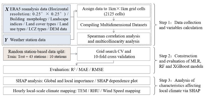
Fig. 1. Workflow of this study.
2.2. Study area
This study was located in Shenzhen, Guangdong Province, China (N22°27'~22°52', E113°46'~114°37'). Shenzhen has a subtropical monsoon climate characterized by long, warm summers and short, mild winters. The climate is mild, with ample sunshine and abundant rainfall. The average annual temperature in Shenzhen is . January has the lowest average temperature at , while July has the highest average temperature at . The average annual precipitation is 1932.9 millimeters, with of the rainfall occurring during the flood season (April to September). Spring weather is variable, dominated by easterly winds. Summer lasts over six months, averaging 202 days, with prevailing southerly winds. In autumn and winter, the northeast monsoon prevails (https://weather.sz.gov.cn/). Additionally, the terrain of Shenzhen is higher in the southeast and lower in the northwest, mostly consisting of low hills interspersed with gentle plateaus. The land cover exhibits high spatial heterogeneity. Its geographical complexity makes it a suitable research area for testing the applicability of machine learning algorithms in predicting air temperature, relative humidity, and wind speed at high spatial and temporal resolutions.
2.3. Data collection and processing
2.3.1. Meteorological data
The total area of Shenzhen is 1997.47 square kilometers. To achieve the goal of downscaling, this study utilized ArcGIS Pro 3.1.0 to create a grid of as the basic analysis unit, covering the entire city of Shenzhen, comprising a total of 2125 grids. These grid units were clipped to fit within Shenzhen's administrative boundaries. The size of the cells was carefully chosen to balance the requirements of computational efficiency and spatial resolution, as shown in Fig. 2(a).
To construct a temperature-humidity-wind mapping model for Shenzhen, meteorological data was collected from the monitoring network of the China Meteorological Administration (CMA). This comprehensive monitoring system comprises both national and regional meteorological stations, adhering strictly to the urban meteorological observation standards set by the World Meteorological Organization (WMO). To ensure the highest standards of data integrity, only data from 53 meteorological stations that provided a complete set of hourly records for one year were selected (Fig. 2(b)). Three key variables were chosen for analysis: near-surface air temperature at a height of 2 meters, relative humidity at 2 meters, and the 2-minute average wind speed at a height of 10 meters. These variables were utilized as dependent variables in the dataset. Furthermore, elevation data for each meteorological station were obtained from the 30-meter resolution NASADEM dataset (https://www.earthdata.nasa.gov/) to represent station altitude as an independent variable.

Fig. 2. Grid system meshed for Shenzhen(a) and the location of weather stations(b).

This study selected various indicators commonly mentioned in urban climate research, including 89 independent variables from six categories, covering ERA5 reanalysis data, building morphology, land use types, land cover types, landscape indices, and LCZ types. All datasets are from the year 2018.
This study used ERA5 reanalysis data as the background meteorological dataset for local-scale climate mapping. ERA5, or the Fifth Generation of the European Centre for Medium-Range Weather Forecasts (ECMWF) Reanalysis (https://cds.climate.copernicus.eu), is a state-of-the-art global atmospheric reanalysis dataset [27]. It provides daily and hourly meteorological parameter data from 1940 to the present. The ERA5 data have a horizontal resolution of and a temporal resolution of 1 hour. Based on existing research, 13 variable parameters were selected to be included in the dataset, and processed using ArcGIS Pro. As shown in Table 1(a), these variables essentially cover the needs of local-scale climate research [28,29].
2.3.2. Built-Environment indicators
Shenzhen is a model of a high-density urban area. The accelerated process of urbanization has led to the formation of over 300 high-rise buildings exceeding 150 meters in height (https://www.skyscrapercenter.com/city/shenzhen), which contributes to a diverse and complex
urban morphology. Incorporating building form into the dataset is crucial for studying the
microclimate impacts in high-density cities [30-32]. To construct the building morphology dataset,
we obtained the building vector data for Shenzhen from an open-source database
(https://zenodo.org/records/8174931) [33]. This study calculated relevant parameters, including
building height, area, volume, and density. Using SAGA GIS 9.5.1, we computed the SVF (Sky
View Factor) for Shenzhen [34]. Road vector data for the year 2018 was sourced from
OpenStreetMap (https://help.openstreetmap.org/) to calculate the Aspect Ratio (AR). In selecting of
data metrics, this study integrates widely used vertical development intensity indicators in the field
of urban planning, such as Total Height (TH) and Height Standard Deviation (HSD), with three-
dimensional morphological indicators, including Total Building Volume (TBV) and Total Building
Surface Area (TBSA). TH and HSD primarily reflect the total vertical development and height
diversity of buildings within urban blocks, while TBV and TBSA are more suitable for measuring
the complexity of three-dimensional building morphology and volume distribution characteristics.
Additionally, density indicators such as Floor Area Ratio (FAR) and Building Coverage Density
(BCD), along with spatial form indicators like Sky View Factor (SVF) and Aspect Ratio (AR), have
been incorporated into the analytical framework to comprehensively assess the development
intensity and spatial environmental characteristics of urban blocks, as shown in Table 1(f).
Different types of land use in urban areas directly influence local climate factors through their
unique thermodynamic and hydrological characteristics. For instance, industrial and transportation
areas, with their extensive impermeable surfaces, are prone to forming heat island cores, while green
spaces regulate the local microclimate through vegetation transpiration and shading effects. The
varying intensity of human activities in commercial and residential areas also affects the spatial
distribution of heat emissions and energy consumption. Therefore, it is essential to incorporate land use types into climate mapping [35]. This study obtained the urban land use data for Shenzhen in 2018 from an open-source database (https://data-starcloud.pcl.ac.cn/zh) [36], as shown in Table 1(b). The percentages of various land use types in each basic analysis unit were calculated and incorporated into the dataset. It not only provided high-precision land use data at a 1-km scale for local-scale climate mapping, but also offered a data basis for quantifying the interaction between urban surface thermal environments and human activities.
Local Climate Zones (LCZ) integrate surface physical properties and human activity characteristics to create a classification system for urban built-up areas with differentiated thermal characteristics [37,38]. Its classification framework comprehensively considers land cover types, three-dimensional morphological parameters, and surface energy balance processes, resulting in a globally applicable quantitative characterization method for urban landscapes [39,40]. This study obtains the LCZ zoning for Shenzhen in 2018 from the LCZ Generator (https://lcz-generator.rub.de/global-locz-map) [41]. Shenzhen has a total of 15 types of LCZ, as shown in Table 1(c). Spatial raster operations were conducted using ArcGIS Pro, and a multidimensional feature dataset was created by calculating the percentage of different LCZ types within each statistical unit. This systemically analyzes the coupling relationship between local-scale climate heterogeneity and spatial morphology.
2.3.3. Land cover types and landscape indices
In urban areas, land cover types play a particularly significant role in evaluating the shaping effects on local climate. Urban land cover patterns, dominated by impervious surfaces, regulate energy balance, intensify the urban heat island effect, and increase near-surface temperatures. The reduction
of vegetation weakens natural cooling and carbon absorption capacities. Combined with artificial heat sources and changes to the urban wind environment, these factors collectively enhance the characteristics of the urban thermal environment. The distribution of impervious surfaces also drives hydrological changes, affecting precipitation runoff and flood risks. Therefore, detailed land cover data can reveal the evolution of urban surface morphology and its climate response mechanisms
[42]. This study obtained 30-meter resolution land cover data from the International Research Center of Big Data for Sustainable Development Goals (https://data.casearth.cn/thematic/glc_fcs30/314)
[43], as shown in Table 1(d). This study calculates the percentage area of different land cover types within the calculation units, providing high-precision data to support the revelation of nonlinear feedback mechanisms between urban surface morphology and local climate systems.
Among the numerous indicators used in landscape pattern research and analysis [44], a selection of representative parameters was chosen, as shown in Table 1(e). These indicators cover the impact of landscape pattern distribution and scale on urban climate [45], such as richness, complexity, and connectivity. Their geometric significance has been detailed in the technical documentation [46] of the FRAGSTATS v4.2 landscape analysis software (https://fragstats.org/) and has been widely discussed in previous studies [47-50]. The landscape metrics required for this study were calculated using the FRAGSTATS v4.2 software, and the values were assigned to the corresponding basic units. This provides high-resolution data to reveal the correlation between urban landscape patterns and local climate [51].
2.4. Spearman correlation analysis and multicollinearity analysis
Data preprocessing is a critical step for enhancing model accuracy. In this study, we initiated the process with Spearman's correlation analysis to identify independent variables significantly
correlated with the dependent variables [52,53]. For each dependent variable, variables with a p
value exceeding 0.01 were excluded to eliminate irrelevant features. A summary of the correlation
analysis between the independent variables and these meteorological indicators is presented in
Figure 3. Subsequently, we addressed multicollinearity by calculating the Variance Inflation Factor
(VIF). Variables exhibiting a VIF greater than 10 were systematically removed. In cases where
multiple variables were found to be collinear, we began with the one possessing the highest VIF.
The correlation strengths of these collinear variables with the dependent variable were then
compared, and the variable demonstrating a weaker correlation was preferentially discarded. This
two-step feature selection process resulted in a refined set of predictors, as shown in Appendix 1:
37 for TEM model, 35 for RHU model, and 38 for Wind Speed model. For model training and
evaluation, the dataset, comprising data from 53 meteorological stations, was partitioned. The
complete annual data (8,760 hours) from a random selection of 43 stations constituted the training
set, whereas data from the remaining 10 stations formed the test set, as shown in Appendix 2. This
station-based partitioning strategy was deliberately chosen to evaluate the model's generalization
performance on geographically unseen locations.
Table 1. Summary of independent variables.


Fig. 3. The Spearman correlation matrix between variables and the T-H-W

(T-H-W: Air temperature, Relative humidity and Wind speed).


2.5. Models
In this study, three models—Multiple Linear Regression (MLR), Random Forest (RF), and Extreme Gradient Boosting (XGBoost)—were initially developed to investigate the complex relationships between various meteorological and environmental parameters and the target variables of air temperature, relative humidity, and wind speed. Notably, the aforementioned models were trained separately and independently for each target variable. MLR served as the baseline model to assess the linear relationships between variables [54]. To account for the prevalent non-linear features in the real world, RF and XGBoost models were further employed to fit these potential non-linear functions. Finally, to quantify and interpret the influence of each input variable from within the complex non-linear models, the SHAP (SHapley Additive exPlanations) method was applied for
model interpretability analysis. This aimed to reveal the specific contribution and impact patterns of each feature on the target variables.
Assuming there are variables in the MLR, namely , in this case, the regression model can be represented as follows in Equation (1):
In the Equation, represents the dependent variable value for individual ( ), denotes the total coefficient of the intercept, represent the total coefficients of the slopes, and is the random error term.
Random Forest is a powerful machine learning technique that predicts values by combining multiple decision trees. It offers robustness against overfitting and improves accuracy by averaging predictions from individual trees [55]. The Random Forest model is trained in Python using the grid search with 10-fold cross-validation to determine the optimal hyperparameter values. The optimal parameters for the air temperature RF model were: max_depth = 7, max_features = 0.8, min_samples_split = 2, and n_estimators = 500. The optimal parameters for the relative humidity RF model were: max_depth = 7, max_features = 0.8, min_samples_split = 2, and n_estimators = 300. The optimal parameters for the wind speed RF model were: max_depth = 7, max_features = 0.8, min_samples_split = 2, and n_estimators = 300.
Extreme Gradient Boosting (XGBoost) is an enhancement of the gradient boosting decision tree (GBDT) algorithm. XGBoost aims to achieve the highest possible speed and efficiency [56]. The XGBoost algorithm, composed of multiple regression trees, can integrate homogeneous weak learners to create a more powerful learner. This can be expressed in Equation (2):
In the equations, represents this study's predicted local climate data, denotes the explanatory variables, and M is the number of trees. refers to the CART tree constructed to reduce the residuals of the tree. The XGBoost model was trained with optimal hyperparameters determined using grid search and 10-fold cross-validation. In the XGBoost training, the optimal parameters for the air temperature XGBoost model were: max_depth = 7, learning_rate = 0.1, n_estimators = 500, colsample_bytree = 0.8, subsample = 0.8. The optimal parameters for the relative humidity XGBoost model were: max_depth = 7, learning_rate = 0.1, n_estimators = 500, colsample_bytree = 0.8, subsample = 0.8. For the wind speed XGBoost model, the optimal parameters were: max_depth = 7, learning_rate = 0.1, n_estimators = 500, colsample_bytree = 0.8, subsample = 0.8.
To evaluate the performance of the model, we used the coefficient of determination , root mean square error (RMSE), and mean absolute error (MAE) as metrics. Formulas (3), (4), and (5) represent the calculations for , RMSE, and MAE, respectively:
2.6. SHAP method
To explain the RF and XGBoost model, SHAP values are used to visualize the relative importance of each variable, which is referred to as the additive feature attribution method [57]. The greatest advantage of SHAP values is that they can represent the influence of features on each sample. For every prediction sample, the model generates a predicted value. SHAP values are assigned to each feature in the sample, indicating both positive and negative influences. The SHAP package could output the feature importance ranking for all samples and creating feature density scatter plots. In the feature importance ranking plot, the X-axis represents SHAP values without distinguishing between positive and negative, while each point in the feature density scatter plot represents a sample. The X-axis indicates SHAP values, where negative (positive) SHAP values represent negative (positive) influence, and the Y-axis value represents the magnitude of the feature variable [58]. The advantage of this method is that it addresses the issue of multicollinearity and considers the synergistic effects of different variables. The functional description of SHAP values for tree-based models is as follows:
where is the SHAP value of the feature , is the set of all features for the training set, the dimension is ; is a permutation subset of , the dimension is , is the average predicted value of samples using the feature set ; is the average predicted value of samples with feature using the feature set , is the weight of the difference between samples with feature and without feature using the feature set .
3. Results
3.1. Model comparisons
3.1.1. Air temperature
Table 2 presents the performance of the MLR, RF, and XGBoost models in air temperature mapping on both the training and testing sets. It is shown that the RF model exhibits the best performance, achieving values of 0.963 and 0.956 for the training and testing sets, respectively. Its MAE and RMSE on the testing set are and , respectively. In contrast, the MLR model performs worse than the RF model, with values of 0.961 and 0.849 for the training and testing sets. The MAE and RMSE on the testing set are and , respectively, which are significantly larger than those of the RF model. Regarding the XGBoost model, although it performs better than the RF model on the training set ( ), its performance on the test set is not as good as the RF model, with an of 0.949, an MAE of , and an RMSE of . To ensure the model adapts well to unseen datasets and to enhance its generalization capability, this study selects the RF model as the training model for air temperature mapping. Fig. 4 illustrates the fitting performance of the three models on the test set.
Table 2. Comparison of fitting ability between training data and testing data of different models for air temperature mapping.

(a) MLR

Fig. 4. The prediction results of MLR, Random Forest and XGBoost models for air temperature mapping (testing data).
(b) RF

(c) XGBoost
To evaluate the model's performance, this study selected ten meteorological stations from the TEM model test set. The results for each station are visualized using a combination of violin plots and box plots. Fig. 7(a) displays the locations of the ten stations in the temperature test set, while Fig. 7(b) presents a detailed distribution of air temperature mapping differences (actual value minus predicted value) for these stations throughout the entire year of 2018, covering a total of 8,760 hours. The results demonstrate that the model exhibits outstanding and consistent performance across all ten test stations. The prediction errors at each station have extremely small median and mean biases, with error distributions highly concentrated—most falling within a narrow range of —indicating the model's high accuracy. Importantly, the error distributions at all stations approximate a symmetric normal distribution centered at zero, a key statistical property suggesting that the model's errors are predominantly random rather than systematic. Furthermore, by considering the station locations in Fig. 7(a), it is evident that this robust performance is maintained across diverse geographical environments, from high-density urban cores to coastal and vegetated areas, fully demonstrating the model's strong spatial generalization capability. Although a small number of extreme outliers exist, the overall analysis confirms the model's high accuracy, reliability, and practical value for high-resolution urban air temperature mapping tasks.
3.1.2. Relative humidity
Table 3 shows the performance of the MLR, RF, and XGBoost models in relative humidity mapping on both the training and testing sets. It is found that XGBoost exhibits the best performance in predicting humidity, achieving values of 0.879 and 0.781 for the training and testing sets, respectively. The MAE and RMSE in the testing set are 5.69% and 7.41%, respectively. The MLR model has values of 0.566 and 0.481 for the training and testing sets, with MAE and RMSE in the testing set being 8.97% and 11.41%, respectively, which are significantly larger than those of the XGBoost model. The RF model has values of 0.670 and 0.642 for the training and testing sets, with MAE and RMSE in the testing set being 7.40% and 9.48%, respectively. Overall, the performance of the MLR and RF models in predicting relative humidity is significantly inferior to that of the XGBoost model. Fig. 5 also illustrates that the fitting effect of the XGBoost model is better than that of the MLR and RF models.
Table 3. Comparison of fitting ability between training data and testing data of different models for relative humidity mapping.

(a) MLR

Fig. 5. The prediction results of MLR, Random Forest and XGBoost models for relative humidity mapping (testing data).
(b) RF

(c) XGBoost
Fig. 7(c) illustrates the locations of the ten stations in the relative humidity test set, while Fig. 7(d)
presents the differences in relative humidity mapping at ten randomly selected stations. The results
indicate that the error analysis of the RHU model reveals a more complex and "station-dependent"
performance characteristic compared to the TEM model. Unlike the relatively consistent
performance of the temperature model, the RHU model exhibits systematic biases of varying
directions and magnitudes across different stations. For example, the model's mean bias fluctuates
considerably among stations, ranging from at station G3678 to at station G3524.
Although the model's performance demonstrates a certain degree of spatial heterogeneity, this does
not obscure its overall high predictive accuracy. Specifically, despite the differences in systematic
bias (mean bias) between stations, the model's predictions within individual stations are highly
consistent, with the majority of error points densely distributed within the range. This
"station-dependent" systematic bias precisely reflects the inherent complexity of high-resolution
urban humidity mapping, which stems from the difficulty in quantifying ultra-local environmental
factors. Therefore, we conclude that the model has successfully captured the macroscopic
distribution patterns of urban humidity, and its demonstrated high accuracy makes it a reliable
analytical tool.
3.1.3. Wind speed
Table 4 shows the performance of the MLR, RF, and XGBoost models in wind speed mapping on
both the training and testing sets. It can be observed that, compared to temperature and relative
humidity, high-resolution wind speed mapping performs poorly, which can be attributed to the
inherently high spatiotemporal variability of wind fields and their sensitivity to local environmental
conditions. In the model comparison, the MLR model completely failed due to its inability to capture nonlinear relationships, resulting in a negative (-0.026) on the test set. Although XGBoost achieved the best performance on the training set , its significant drop in performance on the test set indicates an overfitting issue. In contrast, the RF model demonstrated the best generalization ability and the most robust performance. While its on the training set (0.524) was lower than that of XGBoost, it achieved a higher (0.194) on the test set, as well as lower MAE (0.92 m/s) and RMSE (1.25 m/s) values. Fig. 6 illustrates the fitting results of the three models, showing that the RF model's fitted line is closer to the ideal state. Therefore, the RF model was selected for its most robust predictive performance on unseen data. Although the wind speed model does not match the temperature and humidity models in terms of overall predictive accuracy, this approach still outperforms traditional interpolation methods, which will be further discussed in Section 4.1.
Table 4. Comparison of fitting ability between training data and testing data of different models for wind speed mapping

(a) MLR

Fig. 6. The prediction results of MLR, Random Forest and XGBoost models for wind speed mapping (testing data)
(b) RF

(c) XGBoost
Fig. 7(e) displays the locations of the ten stations in the wind speed test set, while Fig. 7(f) presents
the differences in wind speed mapping at ten randomly selected stations. A key positive finding is
that the model does not exhibit significant systematic bias, as the mean and median prediction errors
at the vast majority of stations are tightly distributed around zero. This indicates that the model has
learned generalizable patterns rather than spurious correlations. The limited score of the model
is mainly attributed to its difficulty in capturing extreme high wind speed events, as evidenced by
the long tails and numerous outliers in the error distributions at all stations. Despite this limitation,
the error patterns show good consistency across stations in different geographic locations,
demonstrating the robust spatial generalization capability of the RF model. In summary, although
the RF model's predictive accuracy for wind speed is limited, its unbiasedness and robust spatial
performance provide a reliable predictive benchmark. The limitation in capturing extreme wind
speed events also highlights a key direction for future model improvement.


Fig. 7. Station-level error analysis of the final models on the independent test set. The figure details the performance of the final models on the held-out test stations. (a), (c), (e) map the geographical locations of the test stations for air temperature, relative humidity, and wind speed, respectively. (b), (d), (f) display the corresponding violin and box plots of the prediction errors ( ), illustrating the error distribution, mean bias, and median bias at each station.

3.2. SHAP analysis
3.2.1. Air temperature analysis
By applying the SHAP model, the SHAP values for each sample feature were calculated. The average of the absolute SHAP values (mean ) was used to display the importance ranking of relevant variables in the air temperature, relative humidity, and wind speed mapping. Due to the
large number of variables, the top 20 variables were selected based on their importance for presentation, and a pie chart was used to illustrate the specific impact proportions of each major category of variables. The average SHAP value represents the average influence of features, with larger values indicating a more significant impact.
Fig. 8 intuitively displays the relative importance ranking of various variables for near-surface air temperature mapping at 2 meters height. Fig. 8(a) shows that ERA5 data makes the most significant contribution to air temperature mapping, accounting for , with the SHAP value of T2M reaching an absolute advantage of 4.3184. LCZ types and building form account for and , respectively, indicating a certain regulatory effect on temperature, while the influence of other data categories is negligible.
Local explanation (Fig. 8(b)) visualizes the SHAP values and directions of the variables. The green and purple dots represent high and low feature values for each variable, respectively. SHAP values greater than zero and less than zero indicate positive and negative influences on hourly air temperature mapping, respectively. Variables such as temperature and the v-component of wind exert positive influences, whereas variables including surface pressure and the land use type characterized by dense trees exhibit negative influences.
This study adopts a systematic analytical approach to deeply explore the nonlinear coupling relationships between temperature and environmental characteristics. The data sources are divided into two main categories: ERA5 reanalysis data and non-ERA5 datasets. Based on SHAP value rankings, the top three key contributing variables were selected for SHAP dependence analysis. As illustrated in Appendix 3(a), the X-axis represents the values of the respective independent variables, while the Y-axis denotes the contribution of each variable to temperature prediction, as quantified
by SHAP values. Among the ERA5 variables, T2M exerts a significant and approximately linear positive effect on temperature mapping, with its SHAP value steadily increasing as the temperature rises. In contrast, the influence of SP is non-linear: when SP is less than , it exhibits a moderately strong positive contribution, whereas beyond this threshold, its effect sharply shifts to a negative correlation. Additionally, SSRD also displays a positive association with temperature prediction; however, the rate of increase in its warming effect markedly diminishes when SSRD exceeds . Regarding the non-ERA5 variables, LCZ11 (proportion of dense trees) generally manifests a slight cooling effect, with its SHAP values predominantly distributed around zero or in the negative range. In comparison, the variables SAD and FAR have minimal impact, as their SHAP values fluctuate closely around the zero line, indicating negligible contributions to temperature prediction.

(a) Global feature importance
Fig. 8. The ranking of importance of the relationship between air temperature mapping and various variables.

(b) Local explanation
3.2.2. Relative humidity analysis
This study quantifies the nonlinear contributions of multi-source environmental variables to the mapping of relative humidity at a height of 2 meters using the SHAP model. Fig. 9(a) shows that ERA5 data has the most significant contribution, accounting for . Local explanation visualizes the SHAP values and directions of the variables, as shown in Fig. 9(b). Variables such as 2m dewpoint temperature, total cloud cover and surface pressure have a positive impact, while variables like surface solar radiation downwards and surface area density have a negative impact.
Next is the SHAP dependence analysis. As shown in Appendix 3(b), this figure illustrates the impact of each variable on relative humidity prediction in the XGBoost model. Among the ERA5 variables, D2M exhibits a significant and approximately linear positive effect on relative humidity mapping, with its SHAP values steadily increasing as the dew point temperature rises. In contrast, SSRD demonstrates a clear negative correlation, with its SHAP values decreasing linearly as radiation intensity increases. TP also shows an important positive effect that its SHAP value rises sharply to a high positive level as precipitation increases from zero, and then climbs more gradually with further increases in precipitation. For the non-ERA5 variables, LCZ11 (proportion of dense trees) displays a clear positive association with relative humidity, indicating that higher tree coverage leads to a stronger humidifying effect. The land use type of residential (101) exhibits a nonlinear influence. As its coverage increases from zero to approximately , its SHAP value rapidly shifts from positive to negative; within the to coverage range, the SHAP value remains stably negative; and when the coverage exceeds , the SHAP value begins to rise, gradually approaching zero. The effect of SAD is relatively complex that it has a slight positive impact in low-density areas , but shifts to a negative correlation in higher-density regions.

(a)Global feature importance
Fig. 9. The ranking of importance of the relationship between relative humidity mapping and various variables.

(b)Local explanation
3.2.3. Wind speed analysis
We examine the nonlinear contributions of variables to the mapping of the 2-minute average wind speed at a height of 10 meters. Fig. 10(a) shows that ERA5 data contributes the most, accounting for . The local explanation visualizes the SHAP values and directions of the variables, as shown in Fig. 10(b). Variables such as the percentage of residential area have a positive impact, whereas variables like surface solar radiation downwards, building height standard deviation, and building floor area ratio exert a negative impact. Due to the influence of wind direction, the U10 and V10 components require separate SHAP dependence analysis.
Next is the SHAP dependence analysis, as shown in Appendix 3(c). In the V10 plot, the north corresponds to positive values and south to negative values. In the U10 plot, east corresponds to positive values and west to negative values. Among the ERA5 data variables, the impact of V10 exhibits a nonlinear pattern. Its SHAP value is positive when the wind direction is southerly, but
turns negative when the wind direction is northerly or weakly southerly, with the critical threshold for this sign change occurring at approximately . In contrast, U10 displays a strong linear negative correlation, with its SHAP value steadily decreasing as the wind direction shifts from westerly to easterly. The effect of SSRD shows that as SSRD increases from 0 to approximately 0.5 , its SHAP value shifts from negative to positive, and then stabilizes at a positive value under higher radiation levels. For non-ERA5 variables, the SHAP value of the land use type for sport and cultural activities (504) drops sharply to a negative value as its coverage increases from 0 to about , and then remains stable. The SHAP value of LCZ11 (dense trees) fluctuates closely around zero throughout the entire coverage range, exhibiting a weakly positive trend. Finally, LCZ4 (open high-rise) shows an initial sharp decline in its SHAP value when the area percentage is less than , but for higher coverage, the SHAP value stabilizes at a level close to zero, indicating a less significant impact compared to other variables.

(a)Global feature importance
Fig. 10. The ranking of importance of the relationship between wind speed mapping and various variables.

(b)Local explanation
3.3. Spatial estimation of local-scale urban climate
In addition to evaluating the overall goodness-of-fit of the model, this study further investigated its performance across specific spatiotemporal dimensions. Fig. 11 visualizes and compares the spatial mapping outcomes of the ERA5 data, the traditional Kriging interpolation method, and the model developed in this study for temperature, relative humidity, and wind speed, using the case of 12:00 PM on the summer solstice in 2018.
Fig. 11(a) focuses on the spatial distribution of air temperature. The ERA5 data exhibit the coarsest spatial resolution, with a grid size of approximately , and are therefore only capable of capturing macroscopic temperature trends at the urban scale. While the Kriging interpolation method produces a smooth and continuous surface and is able to identify several thermal hotspots, its inherent tendency toward over-smoothing obscures the sharp boundaries of temperature variation induced by complex land surface heterogeneity. In contrast, our TEM RF model provides superior spatial detail of the urban thermal environment during the summer solstice noon. It reveals a distinct "west-high, east-low; north-high, south-low" temperature pattern, directly corresponding to Shenzhen's "dense west, sparse east" development. At a finer scale, the model precisely captures the complex thermal landscape of the urban heat island. It identifies the city center as a primary hotspot, distinguishes smaller hot and cool islands linked to building density and land use, and even resolves localized extreme hotspots of . This level of fine-scale differentiation, a product of the complex urban surface, is absent in both ERA5 data and Kriging interpolations.
Similarly, Fig. 11(b) compares the spatial distribution of relative humidity. ERA5's coarse resolution only provides a vague south-to-north gradient. While Kriging outlines the general pattern of higher coastal humidity, its inherent smoothing effect obscures local variations driven by land surface
morphology. In contrast, our RHU XGBoost model successfully captures the city's complex humidity heterogeneity. It accurately reveals that built-up areas are significantly drier than eastern suburbs and ecological lands, a pattern corresponding to the high-temperature zones in Fig. 11(a). Furthermore, the model faithfully depicts the coastal effect, showing narrow coastal zones with the highest relative humidity (94–100%). This fine-scale differentiation, shaped by both urban and natural geography, is beyond the capabilities of ERA5 and Kriging, demonstrating our model's superior performance.
Finally, Fig. 11(c) compares the wind speed mapping results. ERA5 provides an extremely coarse distribution, showing higher wind speeds in the east but failing to capture any internal heterogeneity. While Kriging produces smooth contours, its wind speed patterns are scattered and do not correspond well with the urban morphology. In contrast, our WIND RF model accurately reproduces the complex wind environment within the urban canopy layer. The results clearly show the impedance effect of built-up areas: wind speeds are lower in dense western and central districts but higher in open eastern coastal zones. More importantly, the model captures micro-scale wind variations induced by building layout and surface roughness, presenting a detailed 1 km-scale map closely coupled with the urban fabric. This fine-scale characterization underscores the substantial advantages of our approach.

Fig. 11. Comparison of spatial distribution mapping for air temperature, relative humidity, and wind speed at 12:00 noon on the summer solstice.
4. Discussions
4.1. Model Performance and Comparative Analysis
In recent years, ERA5 data has been widely used in climate research, but its reliability in air temperature, relative humidity, and wind speed mapping has not been fully validated. Barry McNicholl et al. systematically compared temperature differences between ERA5 and the Global Historical Climatology Network (GHCN), a quality-controlled global database of land-based station observations, revealing the seasonal bias characteristics of ERA5[29]. Following this established
validation principle, other researchers have also developed correction methods for various parameters. Kevin Wolf et al. assessed ERA5's performance for upper-atmospheric data and used a bivariate quantile mapping method for calibration [59], while Freddy Houndekindo et al. developed a deep learning framework to correct ERA5 hourly wind speed [60]. Building on this principle of ground-truth validation, this study proposes a framework for combining multi-source heterogeneous data with ERA5 for microclimate mapping, utilizing the authoritative observational data from the China Meteorological Administration (CMA) as the benchmark for our study region.
To validate our methodology, we compared model predictions with ERA5 data resolution) and station observations for 10 test sites, as shown in Table 5. For temperature, the model improved from 0.927 to 0.956, with corresponding decreases in MAE and RMSE. Relative humidity showed a more pronounced gain, with jumping from 0.465 to 0.781. The improvement for wind speed was most notable, its turned positive (0.151) while MAE and RMSE fell to 0.93 m/s and 1.28 m/s. While the absolute wind speed accuracy is not particularly high, this is expected, as coarse ERA5 data cannot resolve site-level variations. Crucially, our goal is not merely to outperform ERA5 but to use it as a reliable, spatiotemporally continuous background field, which we refine with high-resolution urban data to achieve a 1 km resolution. Therefore, our model's superior performance in ground-based validation is an expected outcome. It demonstrates that integrating localized geographic information is essential for accurate downscaling in heterogeneous urban areas.
Table 5. Compare the ERA5 air temperature, relative humidity, and wind speed data at a resolution of from 10 testing stations, along with model predictions and actual meteorological station values (using the best model).
In addition, we selected data from the 10 test set stations at 12:00 noon on the summer solstice of 2018 to quantitatively compare the model predictions with both ERA5 and the traditional Kriging interpolation method. The validation results are presented in Table 6. Both ERA5 and Kriging showed significant limitations against ground observations, yielding negative values. This indicates their inability to capture fine-grained spatiotemporal climate characteristics within heterogeneous urban areas, leading to occasional discrepancies with empirical observations. In contrast, our model achieves a substantial improvement in performance, with values shifting from negative to positive correlations (0.546 for temperature, 0.425 for relative humidity, and 0.221 for wind speed), and significant reductions in MAE and RMSE. Furthermore, the superiority of the model in quantitative metrics is also visually confirmed in Fig. 11.
Table 6. Accuracy validation and comparison of ERA5, Kriging, and the proposed model against ground station measurements at 12:00 noon on the summer solstice.
4.2. Influencing factors
4.2.1. Air temperature
This study conducted a comprehensive analysis of the influence of multiple environmental parameters on temperature mapping. As shown in Fig. 8, ERA5 data contributed the most to
temperature inversion, accounting for , while LCZ types and building form contributed and , respectively. In contrast, the contributions of other types of variables were negligible.
Firstly, by integrating Fig. 8 and Appendix 3(a), it can be observed that the ERA5 exhibits a high contribution. Among these, the SHAP plot confirms a strong linear positive correlation between T2M and the model's contribution. This finding is consistent with the physical understanding that near-surface air temperature is the most direct indicator of the regional thermal environment [61]. In contrast, the second and third most important variables, SP and SSRD, display more complex nonlinear effects. When SP is less than , it has a positive contribution to air temperature, but beyond this threshold, its contribution sharply shifts to a strong negative effect. This may reflect the influence of different weather systems. For example, moderate pressure may correspond to warming under clear skies, whereas high-pressure systems are sometimes associated with cold air activity [62]. Similarly, although SSRD is positively correlated with air temperature, its warming effect becomes saturated at higher radiation levels (above approximately ). This phenomenon aligns with physical principles, as the energy received by the surface, once increased to a certain extent, is dissipated through other processes such as convection and evaporation, thereby limiting the unlimited linear increase in temperature [63].
Although ERA5 variables are predominant, high-resolution non-ERA5 variables are crucial for capturing the fine-scale spatial heterogeneity of temperature. Among all non-ERA5 variables, LCZ11 (Dense Trees) exhibits the most significant impact. Its dependence plot clearly demonstrates that as the coverage of LCZ11 increases, it consistently exerts a slight but stable cooling effect on air temperature. This finding is fully consistent with the well-established mechanism by which vegetation mitigates the urban heat island effect through transpiration and shading [64]. In contrast,
global importance scores for urban morphological indicators such as Surface Area Density (SAD) and Floor Area Ratio (FAR) are relatively low, suggesting that, within the study area and modeling framework, the cooling effect of vegetation cover may be more widespread and pronounced than the direct influence of urban morphological characteristics.
In summary, while ERA5 variables offer a solid foundation for air temperature mapping, incorporating non-ERA5 variables like building morphology or LCZ types helps overcome ERA5's spatial limitations and captures real-world environmental features not represented in physical models, thus improving the accuracy and guidance of temperature mapping models.
4.2.2. Relative humidity
In terms of relative humidity mapping, as shown in Fig. 9, the overall contributions of the different categories of variables are as follows: ERA5 data > LCZ types > land use types > building form > landscape index.
Firstly, by combining Fig. 9 and Appendix 3(b), it can be observed that ERA5 parameters contribute up to to temperature mapping. D2M shows a positive correlation with SHAP values, meaning that as D2M increases, relative humidity also rises. This is because D2M directly reflects the absolute water vapor content in the air; a higher dew point naturally leads to higher relative humidity [65]. In contrast, SSRD shows a clear linear negative correlation. This is because enhanced radiation increases air temperature, thereby raising the air's capacity to hold water vapor. If absolute humidity remains unchanged, this directly results in a decrease in relative humidity [66]. Notably, the effect of TP is characterized by a nonlinear stepwise pattern. Once precipitation occurs , its SHAP value immediately jumps to a higher positive plateau. This suggests that the model has accurately identified the occurrence of precipitation as a key signal for predicting saturated or near-saturated
atmospheric conditions, whose importance far exceeds the actual amount of precipitation [67].
Secondly, analyze the variables from non-ERA5 data. The LCZ11 (dense trees) shows a clear
positive correlation with relative humidity, meaning more tree cover leads to higher humidity. This
is mainly due to plant evapotranspiration, where vegetation releases water vapor into the air,
increasing near-surface humidity and thus raising relative humidity [68]. Residential land
nonlinearly impacts relative humidity. An initial increase in coverage sharply decreases RHU, as
impervious surfaces replace natural landscapes, reducing evapotranspiration and increasing sensible
heat. However, this drying effect diminishes at high densities , suggesting a saturation point
or the compensatory influence of anthropogenic moisture sources [69]. Similarly, SAD is negatively
correlated with relative humidity, particularly in high-density regions (SAD ). This is
because built structures increase sensible heat flux and reduce evaporative surfaces, contributing to
the urban dry island effect [70]. In summary, the mapping of relative humidity is still dominated by
ERA5 data; however, the influence of non-ERA5 variables has made a greater contribution
compared to temperature mapping.
4.2.3. Wind speed
In the mapping of wind speed, as illustrated in Fig. 10, the integrated contributions of various
variables are as follows: ERA5 data land use types LCZ types building form landscape
index DEM.
First, analyze the ERA5 parameters. By integrating the information from Fig. 10 and Appendix 3(c),
it is evident that the 10-metre V-component and U-component of wind emerge as the two most
significant features, and their influence mechanisms directly reflect the model's capacity to learn
the background wind field. The U10 exhibits a linear negative correlation with model predictions.
In contrast, the V10 displays a V-shaped nonlinear effect, where southerly winds contribute positively and northerly winds negatively. This suggests the model captures direction-dependent influences attributable to regional monsoon characteristics and land-sea distribution. SSRD exhibits a stepwise positive influence on wind speed. Its impact becomes positive only after surpassing a key threshold, aligning with its physical role in driving thermal circulations. The model accurately captures that significant solar insolation enhances wind, whereas stable atmospheric conditions under low insolation lead to weaker winds [71].
Secondly, analyze the variables of non-ERA5 categories. High-resolution non-ERA5 variables, especially land use types representing surface roughness, play a crucial role in correcting wind speed. Both the land use type of sport and cultural (504) and LCZ4 (open high-rise buildings) exert a negative influence on near-surface wind. Even minimal coverage introduces significant surface roughness, causing a sharp, stable reduction in wind speed. This suggests their presence, rather than their fractional coverage, is the dominant factor in establishing this obstructive effect at the scale. In contrast, LCZ11 (dense trees) shows a negligible influence, with SHAP values consistently near zero. This suggests that dense trees are a secondary factor for scale wind speed, less critical than dominant drivers in the model. In summary, the contribution of ERA5 variables to wind speed effects decreases, while the contributions of LCZ type, land use type and building form significantly increase, indicating the importance of incorporating non-ERA5 variables in wind speed mapping.
4.3. Comparison to other studies
This study demonstrates the advantages of machine learning in depicting hourly air temperature, relative humidity and wind speed distributions. In terms of hourly air temperature mapping, existing
studies typically achieve root mean square errors (RMSE) and mean absolute errors (MAE) ranging from 0.8 to and 0.6 to , respectively [72,73]. In this study, the RMSE for the hourly temperature mapping test set is and the MAE is , indicating that our model achieves an upper-middle level of performance compared to existing mainstream machine learning studies and demonstrates competitive accuracy. Additionally, for relative humidity mapping, the test set yields an RMSE of and an MAE of , with an of 0.781, which represents a relatively favorable result. Regarding wind speed mapping, although the absolute accuracy of our model is limited, this outcome remains significant given the extreme complexity of wind fields within the urban canopy. In contrast to the negative produced by multiple linear regression (MLR) and the failure of traditional interpolation methods, our model represents a substantial methodological breakthrough. It demonstrates that machine learning approaches are capable of capturing certain nonlinear patterns in wind fields, thereby providing a valuable baseline and perspective for future in-depth research in this challenging domain.
4.4. Potential applications
In recent years, data-driven methods have emerged in the field of weather forecasting, overcoming the challenges of computational efficiency, accuracy, and scalability faced by numerical weather prediction (NWP) systems. Some global data-driven weather forecasting models, such as Pangu-Weather, ClimaX, and Aurora, have already surpassed traditional NWP systems in forecasting accuracy, demonstrating immense application potential [74,75]. However, the accuracy of most large-scale weather forecasting models remains at the mesoscale level (the prediction accuracy of the Pangu model is , approximately 27.5 kilometers), making it difficult to meet the demands of block-scale weather forecasting and predictions in different built environments. This
study aims to leverage multi-source data to bridge the gap between AI-based weather forecasting and high-precision climate prediction, enabling future weather predictions.
The high-resolution local climate mapping proposed in this study offers significant application value. For air temperature, it allows for a more accurate delineation of urban heat island spatial details, providing a scientific basis for health risk assessments and building energy optimization [76]. High-resolution humidity data facilitates the assessment of human thermal comfort, supporting public health interventions and microclimate regulation. Furthermore, refined wind speed data can inform the design of urban ventilation corridors, enhance natural ventilation, and improve air pollution dispersion models. By integrating the synergistic effects of these variables, the dataset provides a more robust decision-making tool for urban planning, environmental health, and energy management, thereby supporting urban climate adaptation and low-carbon development.
4.5. Limitation and future work
There are still limitations in this study that need to be addressed in future studies.
- Spatial scale limitations. The current study only constructs machine learning models at a 1-km scale, while the optimal spatial scale for meteorological parameter retrieval remains worthy of discussion. Future work will involve multi-scale nested experiments to verify how scale effects influence retrieval accuracy. This aligns with research showing that multi-scale approaches using variograms for a priori approximations can significantly improve prediction accuracy in environmental correlation models.
- Temporal generalization limitations. The current training model is based solely on meteorological data from 2018, and while this has validated the feasibility of the methodology, its generalization capability across other years has not been evaluated. Future work will incorporate multi-decadal
data to refine the model and enhance its adaptability to long-term climate fluctuations. This approach is supported by research utilizing extensive historical datasets and physics-informed machine learning to improve temporal generalization capabilities.
- Extreme weather challenges. During extreme weather events such as typhoons, the nonlinear interactions between atmospheric variables significantly intensify, potentially making it difficult for models to provide reliable predictions. Future work requires designing dynamic calibration strategies for such extreme events, such as developing hybrid forecasting frameworks that incorporate WRF model outputs. Research has shown that hybrid approaches combining machine learning with WRF models through spectral nudging techniques have significantly improved the accuracy of typhoon track and intensity forecasts.
- Resource requirements for regional applications. When the model is expanded to a regional scale, the volume of training data will increase dramatically, leading to higher demand on computational resources. Future work can involve ranking feature importance to eliminate redundant variables. This will make the model architecture compatible with variable sets used in mainstream AI weather forecasting systems like ECMWF, enabling effective integration of multi-scale forecasting.
- Limitations of the training target. The weather station data used as ground truth is not free from systematic errors, such as instrumental drift. Training on these observations creates a risk that the model inadvertently learns and reproduces these biases. Future work could mitigate this by integrating diverse data sources, like crowdsourced sensor networks, to create a more robust, bias-corrected target.
- Absence of explicit physical constraints. This study focuses on statistical bias correction and does not incorporate explicit physical constraints into the machine learning model. Future work will
explore the potential of physics-informed neural networks (PINNs) and hybrid frameworks to incorporate governing atmospheric dynamics into the training process, enabling more physically consistent correction of reanalysis outputs.
5. Conclusions
This study developed a comprehensive indicator system utilizing multi-source data to analyze the complex relationships between environmental variables and climate patterns in urban environments. The research integrated multiple data sources from 2018, including the ERA5 reanalysis dataset, building morphology metrics, and landscape indices, creating a multi-dimensional dataset across six categories. It was further combined with temperature-humidity-wind data collected from 53 urban meteorological monitoring stations distributed across Shenzhen, enabling the mapping of these parameters at a 1-km resolution. Using the machine learning model and the SHAP analysis method to explain the nonlinear relationships between variables and temperature-humidity-wind. The main conclusions are as follows:
- The machine learning model demonstrated strong performance in temperature and humidity mapping, achieving high accuracy in predicting air temperature and relative humidity .
- Based on the trained model, this study produced high spatiotemporal resolution (1 km, 1 hour) maps of air temperature, relative humidity, and wind speed for Shenzhen, revealing the spatiotemporal heterogeneity of meteorological elements across the entire city at the 1 km scale.
- This paper applies interpretable machine learning to quantify the importance of the variables used in systematic downscale of meteorological parameters to ). Our feature
importance analysis reveals that the key predictors learned by the models are highly task-specific,
aligning closely with the underlying physics of each target variable. For instance, 2m dewpoint
temperature (D2M) is paramount for the relative humidity mapping, which is expected as RHU is
physically derived from it. In contrast, the air temperature model is overwhelmingly driven by
ERA5's own T2M. Similarly, the wind speed model is dominated by the U10 and V10 wind
components. This task-specific nature of feature importance underscores that our models have
successfully identified the most direct and physically relevant drivers for each microclimate variable.
For non-meteorological parameters, the LCZ types and building form are consistently more
significant than other categories. These findings collectively suggest that successful high-resolution
meteorological downscaling critically depends on the integration of large-scale atmospheric
conditions with small-scale urban morphology.
Despite its promising results, this study has several limitations. The current model is limited to a 1-
km spatial scale and a single year's data, requiring further validation across different spatial
resolutions and extended time periods. Additionally, challenges remain in accurately modeling
extreme weather events and scaling the approach for broader regional applications. Future work will
focus on multi-scale experiments, incorporating multi-year datasets, developing strategies for
extreme events, and optimizing computational efficiency for large-scale use. In addition, the
limitations of the training target and the absence of explicit physical constraints are also limitations
of this study. In summary, this research not only bridges the gap between AI-driven weather
forecasting and high-precision urban climate prediction, but also provides a valuable scientific basis
and decision-making tool for urban heat island analysis, public health risk assessment, building
energy optimization, and climate adaptation planning, highlighting its broad application potential and research significance.
ACKNOWLEDGEMENT
This study was supported by the National Key R&D Program of China (2023YFC3807405)
CONFLICT OF INTEREST
The authors declare no competing interests.
DECLARATION OF GENERATIVE AI AND AI-ASSISTED TECHNOLOGIES IN THE WRITING PROCESS
During the preparation of this work the authors did not use generative AI and/or any AI-assisted technologies in the writing process.
References
[1] T.R. Oke, G. Mills, A. Christen, J.A. Voogt, Urban Climates, 1st ed., Cambridge University Press, 2017. https://doi.org/10.1017/9781139016476.
[2] P. Shen, B. Yang, Projecting Texas energy use for residential sector under future climate and urbanization scenarios: A bottom-up method based on twenty-year regional energy use data, Energy 193 (2020) 116694. https://doi.org/10.1016/j.energy.2019.116694.
[3] K. Deilami, Md. Kamruzzaman, Y. Liu, Urban heat island effect: A systematic review of spatiotemporal factors, data, methods, and mitigation measures, Int. J. Appl. Earth Obs. Geoinformation 67 (2018) 30–42. https://doi.org/10.1016/j.jag.2017.12.009.
[4] P. Shen, Y. Ji, Y. Li, M. Wang, X. Cui, H. Tong, Combined impact of climate change and urban heat island on building energy use in three megacities in China, Energy Build. 331 (2025) 115386. https://doi.org/10.1016/j.enbuild.2025.115386.
[5] G.O. Ofremu, B.Y. Raimi, S.O. Yusuf, B.A. Dziornu, S.G. Nnabuife, A.M. Eze, C.A. Nnajiofor, Exploring the relationship between climate change, air pollutants and human health: Impacts, adaptation, and mitigation strategies, Green Energy Resour. 3 (2025) 100074. https://doi.org/10.1016/j.gerr.2024.100074.
[6] P. Shen, M. Wang, H. Ma, N. Ma, On the two-way interactions of urban thermal environment and air pollution: A review of synergies for identifying climate-resilient mitigation strategies, Build. Simul. 18 (2024) 259–279. https://doi.org/10.1007/s12273-024-1210-x.
[7] M. Viggiano, L. Busetto, D. Cimini, F. Di Paola, E. Geraldi, L. Ranghetti, E. Ricciardelli, F. Romano, A new spatial modeling and interpolation approach for high-resolution temperature maps combining reanalysis data and ground measurements, Agric. For. Meteorol. 276-277 (2019) 107590. https://doi.org/10.1016/j.agrformet.2019.05.021.
[8] J.C. Lo, Z. Yang, R.A. Pielke, Assessment of three dynamical climate downscaling methods using the Weather Research and Forecasting (WRF) model, J. Geophys. Res. Atmospheres 113 (2008) 2007JD009216. https://doi.org/10.1029/2007JD009216.
[9] E. Kalnay, Atmospheric modeling, data assimilation and predictability, 7. print, Cambridge University Press, Cambridge, 2012.
[10] T. Palmer, R. Hagedorn, eds., Predictability of Weather and Climate, 1st ed., Cambridge University Press, 2006. https://doi.org/10.1017/cbo9780511617652.
[11] R. Lam, A. Sanchez-Gonzalez, M. Willson, P. Wirnsberger, M. Fortunato, F. Alet, S. Ravuri, T. Ewalds, Z. Eaton-Rosen, W. Hu, A. Merose, S. Hoyer, G. Holland, O. Vinyals, J. Stott, A. Pritzel, S. Mohamed, P. Battaglia, Learning skillful medium-range global weather forecasting, Science 382 (2023) 1416–1421. https://doi.org/10.1126/science.adi2336.
[12] R.S. Dos Santos, Estimating spatio-temporal air temperature in London (UK) using machine learning and earth observation satellite data, Int. J. Appl. Earth Obs. Geoinformation 88 (2020) 102066. https://doi.org/10.1016/j.jag.2020.102066.
[13] I. Kloog, F. Nordio, B.A. Coull, J. Schwartz, Predicting spatiotemporal mean air temperature using MODIS satellite surface temperature measurements across the Northeastern USA, Remote Sens. Environ. 150 (2014) 132–139. https://doi.org/10.1016/j.rse.2014.04.024.
[14] A. Shtiliyanova, G. Bellocchi, D. Borras, U. Eza, R. Martin, P. Carrère, Kriging-based approach to predict missing air temperature data, Comput. Electron. Agric. 142 (2017) 440–449. https://doi.org/10.1016/j.compag.2017.09.033.
[15] T. Wu, Y. Li, Spatial interpolation of temperature in the United States using residual kriging,
Appl. Geogr. 44 (2013) 112-120. https://doi.org/10.1016/j.apgeog.2013.07.012.
[16] X. Ding, Y. Zhao, Y. Fan, Y. Li, J. Ge, Machine learning-assisted mapping of city-scale air temperature: Using sparse meteorological data for urban climate modeling and adaptation, Build. Environ. 234 (2023) 110211. https://doi.org/10.1016/j.buildenv.2023.110211.
[17] G. Chen, Y. Shi, R. Wang, C. Ren, E. Ng, X. Fang, Z. Ren, Integrating weather observations and local-climate-zone-based landscape patterns for regional hourly air temperature mapping using machine learning, Sci. Total Environ. 841 (2022) 156737. https://doi.org/10.1016/j.scitotenv.2022.156737.
[18] H. Shen, Y. Jiang, T. Li, Q. Cheng, C. Zeng, L. Zhang, Deep learning-based air temperature mapping by fusing remote sensing, station, simulation and socioeconomic data, Remote Sens. Environ. 240 (2020) 111692. https://doi.org/10.1016/j.rse.2020.111692.
[19] T. Li, X. Zheng, Y. Dai, C. Yang, Z. Chen, S. Zhang, G. Wu, Z. Wang, C. Huang, Y. Shen, R. Liao, Mapping near-surface air temperature, pressure, relative humidity and wind speed over Mainland China with high spatiotemporal resolution, Adv. Atmospheric Sci. 31 (2014) 1127-1135. https://doi.org/10.1007/s00376-014-3190-8.
[20] N. Nikolaou, L.M. Bouwer, M. Dallavalle, M. Valizadeh, M. Stafoggia, A. Peters, K. Wolf, A. Schneider, Improved daily estimates of relative humidity at high resolution across Germany: A random forest approach, Environ. Res. 238 (2023) 117173. https://doi.org/10.1016/j.envres.2023.117173.
[21] G. Chen, J. Hua, Y. Shi, C. Ren, Constructing air temperature and relative humidity-based hourly thermal comfort dataset for a high-density city using machine learning, Urban Clim. 47 (2023) 101400. https://doi.org/10.1016/j.uclim.2022.101400.
[22] Z. Liu, P. Jiang, L. Zhang, X. Niu, A combined forecasting model for time series: Application to short-term wind speed forecasting, Appl. Energy 259 (2020) 114137. https://doi.org/10.1016/j.apenergy.2019.114137.
[23] Z. Zhang, L. Lin, S. Gao, J. Wang, H. Zhao, H. Yu, A machine learning model for hub-height short-term wind speed prediction, Nat. Commun. 16 (2025). https://doi.org/10.1038/s41467-025-58456-4.
[24] C. Huang, J. Yao, B. Fu, J.K. Calautit, C. Zhao, J. Huang, Q. Ban, Sensitivity analysis of WRF-CFD-based downscaling methods for evaluation of urban pedestrian-level wind, Urban Clim. 49 (2023) 101569. https://doi.org/10.1016/j.uclim.2023.101569.
[25] X. Wang, C. Hu, H. Kikumoto, H. Jia, K. Nakao, R. Ooka, Data extension of high-resolution wind speed database by fusing meteorological observation and local objective analysis data with POD-LSE, J. Wind Eng. Ind. Aerodyn. 252 (2024) 105812. https://doi.org/10.1016/j.jweia.2024.105812.
[26] P. Shen, J. Liu, M. Wang, Fast generation of microclimate weather data for building simulation under heat island using map capturing and clustering technique, Sustain. Cities Soc. 71 (2021) 102954. https://doi.org/10.1016/j.scs.2021.102954.
[27] Hersbach H, Bell B, Berrisford P, Biavati G, Horányi A, Muñoz Sabater J, Nicolas J, Peubey C, Radu R, Rozum I, Schepers D, ERA5 hourly data on single levels from 1940 to present, (2018). https://doi.org/10.24381/CDS.ADBB2D47.
[28] D.H. Klinges, J.P. Duffy, M.R. Kearney, I.M.D. Maclean, MCERA5: Driving microclimate models with ERA5 global gridded climate data, Methods Ecol. Evol. 13 (2022) 1402-1411. https://doi.org/10.1111/2041-210x.13877.
[29] B. McNicholl, Y.H. Lee, A.G. Campbell, S. Dev, Evaluating the Reliability of Air Temperature From ERA5 Reanalysis Data, IEEE Geosci. Remote Sens. Lett. 19 (2022) 1-5. https://doi.org/10.1109/lgrs.2021.3137643.
[30] F. Biljecki, Y.S. Chow, Global Building Morphology Indicators, Comput. Environ. Urban Syst. 95 (2022) 101809. https://doi.org/10.1016/j.compenvurbsys.2022.101809.
[31] H. Li, Y. Li, T. Wang, Z. Wang, M. Gao, H. Shen, Quantifying 3D building form effects on urban land surface temperature and modeling seasonal correlation patterns, Build. Environ. 204 (2021) 108132. https://doi.org/10.1016/j.buildenv.2021.108132.
[32] Y. Ming, Y. Liu, Y. Li, Y. Song, Unraveling nonlinear and spatial non-stationary effects of urban form on surface urban heat islands using explainable spatial machine learning, Comput. Environ. Urban Syst. 114 (2024) 102200. https://doi.org/10.1016/j.compenvurbsys.2024.102200.
[33] Q. Shi, Jiajun Zhu, Zhengyu Liu, Haonan Guo, Mengxi Liu, Zihong Liu, Xiaoping Liu, A first high-quality vector data of buildings in East Asian countries based on a comprehensive large-scale mapping framework, (2023). https://doi.org/10.5281/ZENODO.8174931.
[34] O. Conrad, B. Bechtel, M. Bock, H. Dietrich, E. Fischer, L. Gerlitz, J. Wehberg, V. Wichmann, J. Böhner, System for Automated Geoscientific Analyses (SAGA) v. 2.1.4, Geosci. Model Dev. 8 (2015) 1991–2007. https://doi.org/10.5194/gmd-8-1991-2015.
[35] W. Li, Y. Bai, Q. Chen, K. He, X. Ji, C. Han, Discrepant impacts of land use and land cover on urban heat islands: A case study of Shanghai, China, Ecol. Indic. 47 (2014) 171-178. https://doi.org/10.1016/j.ecolind.2014.08.015.
[36] P. Gong, B. Chen, X. Li, H. Liu, J. Wang, Y. Bai, J. Chen, X. Chen, L. Fang, S. Feng, Y. Feng, Y. Gong, H. Gu, H. Huang, X. Huang, H. Jiao, Y. Kang, G. Lei, A. Li, X. Li, X. Li, Y. Li, Z. Li, Z. Li, C. Liu, C. Liu, M. Liu, S. Liu, W. Mao, C. Miao, H. Ni, Q. Pan, S. Qi, Z. Ren, Z. Shan, S. Shen, M. Shi, Y. Song, M. Su, H. Ping Suen, B. Sun, F. Sun, J. Sun, L. Sun, W. Sun, T. Tian, X. Tong, Y. Tseng, Y. Tu, H. Wang, L. Wang, X. Wang, Z. Wang, T. Wu, Y. Xie, J. Yang, J. Yang, M. Yuan, W. Yue, H. Zeng, K. Zhang, N. Zhang, T. Zhang, Y. Zhang, F. Zhao, Y. Zheng, Q. Zhou, N. Clinton, Z. Zhu, B. Xu, Mapping essential urban land use categories in China (EULUC-China): preliminary results for 2018, Sci. Bull. 65 (2020) 182–187. https://doi.org/10.1016/j.scib.2019.12.007.
[37] M. Demuzere, J. Kittner, B. Bechtel, LCZ Generator: A Web Application to Create Local Climate Zone Maps, Front. Environ. Sci. 9 (2021). https://doi.org/10.3389/fenvs.2021.637455.
[38] P. Shen, Spatiotemporal mapping of urban air temperature and UHI under TMY condition: A reference station based machine learning approach, Energy Build. 343 (2025) 115923. https://doi.org/10.1016/j.enbuild.2025.115923.
[39] X. Chen, W. Tu, J. Yu, R. Cao, S. Yi, Q. Li, LCZ-based city-wide solar radiation potential analysis by coupling physical modeling, machine learning, and 3D buildings, Comput. Environ. Urban Syst. 113 (2024) 102176. https://doi.org/10.1016/j.compenvurbsys.2024.102176.
[40] F. Hashemi, G. Mills, U. Poerschke, L.D. Iulo, G. Pavlak, L. Kalisperis, A novel parametric workflow for simulating urban heat island effects on residential building energy use: Coupling local climate zones with the urban weather generator a case study of seven U.S. cities, Sustain. Cities Soc. 110 (2024) 105568. https://doi.org/10.1016/j.scs.2024.105568.
[41] M. Demuzere, J. Kittner, A. Martilli, G. Mills, C. Moede, I.D. Stewart, J. Van Vliet, B. Bechtel, A global map of local climate zones to support earth system modelling and urban-scale environmental science, Earth Syst. Sci. Data 14 (2022) 3835–3873. https://doi.org/10.5194/essd-14-3835-2022.
[42] X. Yang, Y. Zhang, L. Liu, W. Zhang, M. Ding, Z. Wang, Sensitivity of surface air temperature change to land use/cover types in China, Sci. China Ser. Earth Sci. 52 (2009) 1207-1215. https://doi.org/10.1007/s11430-009-0085-0.
[43] X. Zhang, T. Zhao, H. Xu, W. Liu, J. Wang, X. Chen, L. Liu, GLC_FCS30D: the first global land-cover dynamics monitoring product with a fine classification system for the period from 1985 to 2022 generated using dense-time-series Landsat imagery and the continuous change-detection method, Earth Syst. Sci. Data 16 (2024) 1353-1381. https://doi.org/10.5194/essd-16-1353-2024.
[44] A. Chen, L. Yao, R. Sun, L. Chen, How many metrics are required to identify the effects of the landscape pattern on land surface temperature?, Ecol. Indic. 45 (2014) 424-433. https://doi.org/10.1016/j.ecolind.2014.05.002.
[45] B. Li, X. Shi, H. Wang, M. Qin, Analysis of the relationship between urban landscape patterns and thermal environment: a case study of Zhengzhou City, China, Environ. Monit. Assess. 192 (2020). https://doi.org/10.1007/s10661-020-08505-w.
[46] K. McGarigal, B.J. Marks, FRAGSTATS: spatial pattern analysis program for quantifying landscape structure., U.S. Department of Agriculture, Forest Service, Pacific Northwest Research Station, Portland, OR, 1995. https://doi.org/10.2737/pnw-gtr-351.
[47] S. Du, Z. Xiong, Y.-C. Wang, L. Guo, Quantifying the multilevel effects of landscape composition and configuration on land surface temperature, Remote Sens. Environ. 178 (2016) 84-92. https://doi.org/10.1016/j.rse.2016.02.063.
[48] H. Li, J. Wu, Use and misuse of landscape indices, Landsc. Ecol. 19 (2004) 389-399. https://doi.org/10.1023/b:land.0000030441.15628.d6.
[49] J. Peng, Y. Wang, Y. Zhang, J. Wu, W. Li, Y. Li, Evaluating the effectiveness of landscape metrics in quantifying spatial patterns, Ecol. Indic. 10 (2010) 217-223. https://doi.org/10.1016/j.ecolind.2009.04.017.
[50] E. Uuemaa, Ü. Mander, R. Marja, Trends in the use of landscape spatial metrics as landscape indicators: A review, Ecol. Indic. 28 (2013) 100–106. https://doi.org/10.1016/j.ecolind.2012.07.018.
[51] L. Lin, Y. Zhao, J. Zhao, Optimizing urban green space spatial patterns for thermal environment improvement: A multi-objective approach in the context of urban renewal, Comput. Environ. Urban Syst. 121 (2025) 102320. https://doi.org/10.1016/j.compenvurbsys.2025.102320.
[52] D. Zwillinger, S. Kokoska, CRC standard probability and statistics tables and formulae, Chapman & Hall/CRC, Boca Raton, 2000.
[53] M.G. Kendall, A. Stuart, The Advanced Theory of Statistics. Vol. 3., Biometrics 25 (1969) 435. https://doi.org/10.2307/2528806.
[54] G.Y. Oukawa, P. Krecl, A.C. Targino, Fine-scale modeling of the urban heat island: A comparison of multiple linear regression and random forest approaches, Sci. Total Environ. 815 (2022) 152836. https://doi.org/10.1016/j.scitotenv.2021.152836.
[55] F. Guo, Q. Wu, U. Schlink, 3D building configuration as the driver of diurnal and nocturnal land surface temperatures: Application in Beijing's old city, Build. Environ. 206 (2021) 108354. https://doi.org/10.1016/j.buildenv.2021.108354.
[56] C. Wegener, C.C. Ibebuchi, Application of XGBoost in Disentangling the Fingerprints of Global Warming and Decadal Climate Modes on Seasonal Precipitation Trends in Ohio, Int. J. Climatol. 45 (2025). https://doi.org/10.1002/joc.8829.
[57] L. Han, J. Zhao, Y. Gao, Z. Gu, Prediction and evaluation of spatial distributions of ozone and
urban heat island using a machine learning modified land use regression method, Sustain. Cities Soc. 78 (2022) 103643. https://doi.org/10.1016/j.scs.2021.103643.
[58] A.B. Parsa, A. Movahedi, H. Taghipour, S. Derrible, A. (Kouros) Mohammadian, Toward safer highways, application of XGBoost and SHAP for real-time accident detection and feature analysis, Accid. Anal. Prev. 136 (2020) 105405. https://doi.org/10.1016/j.aap.2019.105405.
[59] K. Wolf, N. Bellouin, O. Boucher, S. Rohs, Y. Li, Correction of temperature and relative humidity biases in ERA5 by bivariate quantile mapping: Implications for contrail classification, (2023). https://doi.org/10.5194/egusphere-2023-2356.
[60] T.B.M.J. Ouarda, F. Houndekindo, LSTM and Transformer-based framework for bias correction of ERA5 hourly wind speeds, (2025). https://doi.org/10.2139/ssrn.5125439.
[61] P.D. Jones, M. New, D.E. Parker, S. Martin, I.G. Rigor, Surface air temperature and its changes over the past 150 years, Rev. Geophys. 37 (1999) 173–199. https://doi.org/10.1029/1999RG900002.
[62] H. Feidas, T. Makrogiannis, E. Bora-Senta, Trend analysis of air temperature time series in Greece and their relationship with circulation using surface and satellite data: 1955?2001, Theor. Appl. Climatol. 79 (2004) 185-208. https://doi.org/10.1007/s00704-004-0064-5.
[63] H. Zhang, Q. Yin, T. Nakajima, N.M. Makiko, P. Lu, J. He, Influence of changes in solar radiation on changes of surface temperature in China, Acta Meteorol. Sin. 27 (2013) 87-97. https://doi.org/10.1007/s13351-013-0109-8.
[64] A. Liu, C. Wang, G. Shang, B. Hong, Assessing tree canopy cooling efficiency in different local climate zones: A cost-benefit analysis, Urban For. Urban Green. 105 (2025) 128694. https://doi.org/10.1016/j.ufug.2025.128694.
[65] M.G. Lawrence, The Relationship between Relative Humidity and the Dewpoint Temperature in Moist Air: A Simple Conversion and Applications, Bull. Am. Meteorol. Soc. 86 (2005) 225-234. https://doi.org/10.1175/bams-86-2-225.
[66]A. Sozen, E. Arcakliog'lu, Effect of relative humidity on solar potential, Appl. Energy 82 (2005) 345-367. https://doi.org/10.1016/j.apenergy.2004.12.001.
[67] E. Eccel, Estimating air humidity from temperature and precipitation measures for modelling applications, Meteorol. Appl. 19 (2012) 118-128. https://doi.org/10.1002/met.258.
[68] Z. Zhang, Y. Lv, H. Pan, Cooling and humidifying effect of plant communities in subtropical urban parks, Urban For. Urban Green. 12 (2013) 323-329. https://doi.org/10.1016/j.ufug.2013.03.010.
[69] S.M. Ahmed, F.K.M. Al-Ramahi, Evaluate the Effect of Relative Humidity in the Atmosphere of Baghdad City urban expansion Using Remote Sensing Data, Iraqi J. Sci. (2022) 1848–1859. https://doi.org/10.24996/ijs.2022.63.4.41.
[70] Y. Jiang, C. Wu, M. Teng, Impact of Residential Building Layouts on Microclimate in a High Temperature and High Humidity Region, Sustainability 12 (2020) 1046. https://doi.org/10.3390/su12031046.
[71] T.-P. Chang, F.-J. Liu, H.-H. Ko, M.-C. Huang, Oscillation characteristic study of wind speed, global solar radiation and air temperature using wavelet analysis, Appl. Energy 190 (2017) 650-657. https://doi.org/10.1016/j.apenergy.2016.12.149.
[72] B. Zhou, E. Erell, I. Hough, J. Rosenblatt, A.C. Just, V. Novack, I. Kloog, Estimating near-surface air temperature across Israel using a machine learning based hybrid approach, Int. J. Climatol. 40 (2020) 6106-6121. https://doi.org/10.1002/joc.6570.
[73] Z. Zhang, Q. Du, Hourly mapping of surface air temperature by blending geostationary datasets
from the two-satellite system of GOES-R series, ISPRS J. Photogramm. Remote Sens. 183 (2022) 111-128. https://doi.org/10.1016/j.isprsjprs.2021.10.022.
[74] I. Price, A. Sanchez-Gonzalez, F. Alet, T.R. Andersson, A. El-Kadi, D. Masters, T. Ewalds, J. Stott, S. Mohamed, P. Battaglia, R. Lam, M. Willson, GenCast: Diffusion-based ensemble forecasting for medium-range weather, (2024). https://doi.org/10.48550/arXiv.2312.15796.
[75] A. Allen, S. Markou, W. Tebbutt, J. Requeima, W.P. Bruinsma, T.R. Andersson, M. Herzog, N.D. Lane, M. Chantry, J.S. Hosking, R.E. Turner, End-to-end data-driven weather prediction, Nature 641 (2025) 1172–1179. https://doi.org/10.1038/s41586-025-08897-0.
[76] P. Shen, Y. Li, X. Gao, S. Chen, X. Cui, Y. Zhang, X. Zheng, H. Tang, M. Wang, Climate adaptability of building passive strategies to changing future urban climate: A review, Nexus 2 (2025) 100061. https://doi.org/10.1016/j.ynexs.2025.100061.
Appendix
Appendix 1. Selected Feature Variables for Model Training
To construct robust and efficient predictive models, a rigorous feature selection process was applied to the initial set of variables. This process involved Spearman Correlation Analysis to assess the monotonic relationship between each variable and the target parameters (temperature, humidity, and wind speed), followed by Multicollinearity Analysis to eliminate redundant features that were highly correlated with each other.
The table below details the final feature variables selected through this process for training the three independent models. The Temperature (TEM) model includes 37 variables, the Relative Humidity (RHU) model includes 35 variables, and the Wind Speed model includes 38 variables.
Appendix 1. Variables Selected via Spearman Correlation and Multicollinearity Analysis
Appendix 2: Partition of Training and Test Stations
To rigorously evaluate the model's spatial generalization performance, a station-based partitioning strategy was employed. This approach ensures that the model is tested on geographically unseen locations, providing a robust assessment of its real-world applicability.
From the total of 53 meteorological stations, 43 were randomly selected to form the training set,
using their complete annual data (8,760 hours). The data from the remaining 10 stations constituted the test set. The table below lists the specific IDs of these 10 test stations. As this random selection was conducted independently for each of the three models, the station lists differ accordingly.
Appendix 2. Sampling results for the test set stations (10 each for the Temperature, Relative Humidity, and Wind Speed models)
Appendix 3. SHAP Dependence Plots for Key Feature Interpretation
To provide deeper insight into the behavior of the "black-box" models (such as RF and XGBoost), we employed the SHAP (SHapley Additive exPlanations) framework for model interpretability. SHAP quantifies the contribution of each feature to individual predictions, revealing the complex non-linear patterns and interaction effects learned by the model. This appendix presents the SHAP dependence plots for the most influential variables in the (a) air temperature, (b) relative humidity, and (c) wind speed models. The variables shown were selected based on their high mean absolute SHAP values (mean (|SHAP value|) and are categorized by their data source (ERA5 vs non-ERA5). How to interpret a SHAP dependence plot:
X-axis: Shows the actual value of a feature.
- Y-axis: Shows the SHAP value for that feature. It indicates how much that feature's value contributes to pushing a specific prediction away from the baseline (average) prediction. A positive SHAP value increases the prediction, while a negative value decreases it.
Each dot: Represents a single instance (sample) from the dataset.
Color: The color illustrates the value of a second feature that has the strongest interaction with
the feature on the x-axis. In these plots, green corresponds to a high value of the interacting feature, while magenta indicates a low value.
Vertical Scatter: The vertical dispersion of the dots reveals interaction effects. A wider spread signifies that the impact of the primary feature is being modified by other features.


(a) SHAP dependence plots for variables in air temperature mapping. (Top 3 |SHAP value|, RF model)


(b) SHAP dependence plots for variables in relative humidity mapping. (Top 3 |SHAP value|, XGBoost model)


(c) SHAP dependence plots for variables in wind speed mapping.

(Top 3 |SHAP value|, RF model)

Appendix 3. SHAP dependence plots for variables. (Top 3 |SHAP value| for ERA5 and non-ERA5 parameters)
Declaration of interest statement
We declare that we have no financial and personal relationships with other people or organizations that can inappropriately influence our work, there is no professional or other personal interest of any nature or kind in any product, service and/or company that could be construed as influencing the position presented in, or the review of, the manuscript entitled "High-resolution spatiotemporal mapping from ERA5 reanalysis: integrating multi-source data with machine learning for the city of Shenzhen".
Workflow of this study
Publication Details
Journal
Building and Environment
Publication Year
2026
Authors
Haida Tang , Jiayu Chen , Xingkang Chai , Chunying Li ,Chunchun Meng , Siyuan Chen , Wei Gu , Pengyuan Shen
Categories
Urban climate and building adaptation strategies