
RCBldGH: Integrating enhanced RC thermal networks to parametric modeling and design for rapid building energy simulation and optimization
Zhenyu Pan, Ang Lu, Pengyuan Shen
2026
Expert Systems with Applications
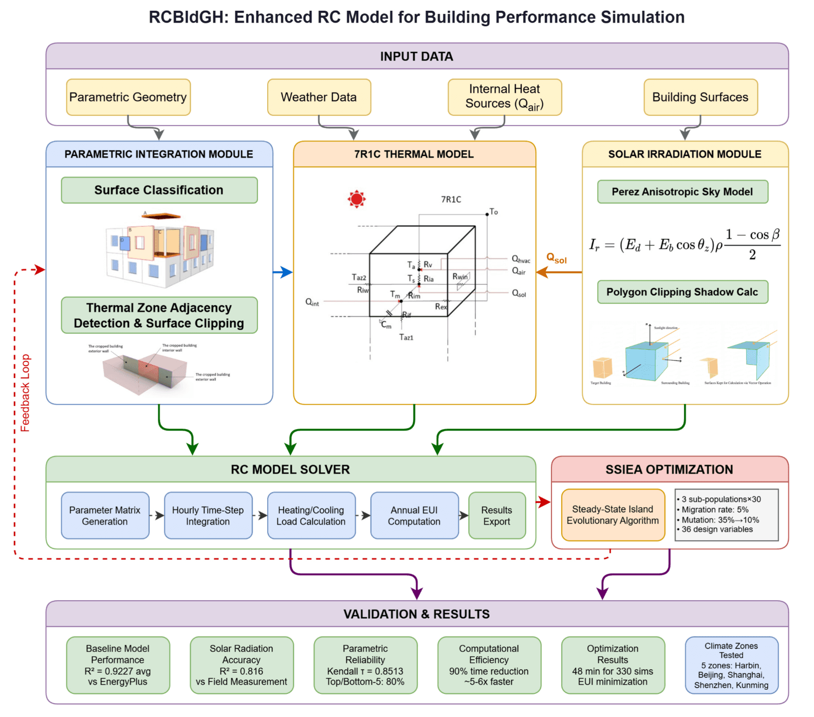
Fig. 1. Flowchart of the parametric design platform for performance optimization with an integrated RC model.
Summary
This study develops RCBldGH, a Grasshopper plugin integrating an enhanced 7R1C grey-box RC thermal network with the Perez sky model for fast building energy prediction. It automates parametric geometry conversion and shading calculation, cutting computation time by nearly 90% vs EnergyPlus. Validated across five Chinese climates, the model achieves an average R² of 0.92 and consistent performance ranking. Coupled with SSIEA evolutionary algorithm, it enables early-stage building form optimization, though it lacks latent heat calculation and has systematic load biases.
Abstract
Architectural design is a critical factor in achieving carbon neutrality goals in the building sector, but its significant emission reduction potential for buildings remains largely unrealized due to the lack of rapid, reliable performance simulation tools in the early design stage. This study introduces an efficient, hybrid grey-box model by coupling an enhanced resistance–capacitance (RC) network model together with Perez sky model and polygon-clipping algorithm for building facade solar irradiance calculation. The model enhanced robustness to design variations and physical interpretability while keeping computational efficiency. Validation across typical building models in multiple climate zones demonstrates high agreement with industry-standard EnergyPlus predictions, achieving a mean R2 of 0.92 with a 90% reduction in computational cost. This work wrapped the model into RCBldGH, an energy calculation plugin in the mainstream 3D modeling software Rhino. The incorporation of a parameter optimization process based on the SSIEA demonstrates the tool’s effectiveness in design space exploration and the identification of optimal design parameter combinations, providing architects and researchers with a rapid iteration energy assessment tool for the early design stage. By embedding RC-based building performance analysis into the parametric design workflow, this tool reduces the complexity of performance-driven building form exploration during early design stages, which offers a practical approach for performance-driven building design exploration.
1. Introduction
The building sector accounts for approximately 36–39% of global carbon emissions (Hu et al., 2025; Rock ¨ et al., 2023), making it critical for achieving carbon neutrality goals (Idrissi Kaitouni et al., 2000; Chen et al., 2022; Shin et al., 2025; Too et al., 2022; Liu et al., 2025). Architectural decisions during early design stages—including building form, orientation, envelope parameters, and passive/active technology integration—exert pivotal influence on lifecycle energy consumption and carbon emissions (Jørgensen and Ma, 2025; Ma et al., 2023; Li et al., 2022; Feng et al., 2025), yet the sector's emission reduction potential remains largely unrealized due to lack of rapid, reliable performance simulation tools supporting iterative design exploration.
Designers require tools capable of rapidly evaluating performance across alternative design options, but existing building performance simulation (BPS) approaches face fundamental trade-offs. Traditional white-box models (EnergyPlus, TRNSYS) achieve high fidelity but require complex inputs and substantial computation that preclude rapid iteration (Coakley et al., 2014). Data-driven black-box models enable near-real-time prediction but exhibit poor generalization beyond training data and lack physical interpretability (Loonen et al., 2017). Grey-box models based on resistance–capacitance (RC) networks offer promising middle ground but face limitations in solar heat gain calcu lation and parametric design integration that constrain practical application (Zhang et al., 2023; Lou et al., 2025). This study addressed those limitations by developing an enhanced RC model integrated into the Grasshopper parametric platform, enabling rapid, reliable performance evaluation during the design exploration process.
2. Literature review
2.1. Building performance simulation approaches
Building performance simulation (BPS) methodologies can be broadly categorized into three paradigms: white-box, black-box, and grey-box models, each representing distinct trade-offs between physical fidelity, computational efficiency, and practical applicability (Li et al., 2021).
White-box models are grounded in first-principles physics, employ ing detailed mathematical representations of heat transfer, mass balances, and thermodynamic processes. Representative tools include EnergyPlus, TRNSYS, and DOE-2, which solve coupled differential equations governing conduction, convection, radiation, and airflow. These models have been extensively validated against experimental data and are widely recognized as industry-standard benchmarks for building energy simulations (Shahcheraghian et al., 2024; Hong et al., 2018). EnergyPlus, developed by the US Department of Energy, incorporates sophisticated algorithms, including conduction transfer function (CTF), the TARP convection model, and detailed fenestration calculations (Magni et al., 2021). TRNSYS offers modular flexibility for system-level simulations and has been applied in solar thermal systems, HVAC optimizations, and renewable energy integration studies (Loonen et al., 2017). These tools have enabled significant advances in building science research and have been adopted into building codes and standards development worldwide (Crawley et al., 2008).
Black-box models leverage statistical learning and machine learning techniques to establish input–output mappings without explicit physical modeling. Artificial neural networks (ANNs) have been applied to predict building energy consumption based on weather data, occupancy patterns, and building characteristics (Roman et al., 2020). Support vector machines (SVMs) have demonstrated effectiveness in forecasting short-term building loads (Kaytez et al., 2015). More recently, deep learning architectures including recurrent neural networks (RNNs) and long short-term memory (LSTM) networks have been employed for time series energy prediction (Luo and Oyedele, 2021; Waheed and Xu, 2025). Gradient boosting methods such as XGBoost have shown strong performance in building energy benchmark applications. These datadriven approaches have been successfully deployed in building energy management systems, demand response programs, and smart grid ap plications, where historical operational data is abundant (Li et al., 2025; Cheng and Yu, 2019).
Grey-box models represent a hybrid paradigm that combines simplified physical structure with data-driven parameter identification. Among grey-box approaches, resistance–capacitance (RC) network models have emerged as particularly promising for building thermal simulation (Beli´c et al., 2021). The RC approach abstracts building thermal dynamics using electrical circuit analogies, where thermal resistance (R) represents heat transfer paths and thermal capacitance C represents heat storage elements. This formulation has been extensively developed for building applications. RC models have been successfully applied in model predictive control (MPC) systems, building energy management, and district heating optimization (Macia ` Cid et al., 2024; Zheng et al., 2024). The ISO 13790 standard has codified simplified RC methods for building energy calculations, establishing their acceptance in regulatory frameworks (Vivian et al., 2017; Maccarini et al., 2021).
2.2. RC network models in building thermal simulation
The development of RC network models for building applications has progressed through several stages, with increasing sophistication in model structure and parameter identification methods (Wang et al., 2019; Wang et al., 2022). The RC approach abstracts building thermal dynamics using electrical circuit analogies, where thermal resistance represents heat transfer paths and thermal capacitance represents heat storage elements. This formulation results in analytically solvable linear differential equations that substantially reduce computational cost and convergence difficulty compared to finite difference and finite element methods (Yang et al., 2024). Early work focused on simple first order models for single zone buildings, which were subsequently extended to multi node configurations capable of representing more complex thermal dynamics.
Model complexity can be varied from simple 2R1C configurations to more sophisticated 7R2C or higher order networks, enabling calibration to specific accuracy requirements. Lower order models are typically employed in Model Predictive Control applications where computational speed is paramount and real time operation is required (Wang et al., 2022; Bacher and Madsen, 2011). Harb and Boyanov demonstrated that 3R2C models can achieve acceptable accuracy for fore casting thermal response with proper parameter identification. Higher order models are preferred for energy simulation tasks requiring greater fidelity, particularly when capturing dynamic thermal mass effects is important. Recent comprehensive reviews indicate that the accuracy of third order or higher RC models does not improve significantly compared to lower order alternatives for many practical applications, suggesting that model selection should balance complexity against computational demands (Yang et al., 2024).
Parameter identification for RC models has been addressed through various approaches. The ISO 13790 standard has codified simplified RC methods for building energy calculations, establishing their acceptance in regulatory frameworks and providing standardized parameter definitions (Vivian et al., 2017; Maccarini et al., 2021; Marty-Jourjon et al., 2022). Unscented Kalman filtering methods have been applied to esti mate RC parameters from measured data while quantifying uncertainty (Chen et al., 2021). Genetic algorithms and particle swarm optimization have been used for parameter optimization against monitored building data (Wang et al., 2019). More recently, physics informed neural networks have been combined with RC model structures to improve parameter estimation accuracy (Chen et al., 2023).
Solar heat gain treatment in RC networks has evolved from simple constant coefficients to more sophisticated approaches. Early implementations used fixed solar gain coefficients or monthly average values (Tamm et al., 2020; Díaz-Hernandez ´ et al., 2020; Mathews et al., 1994). Direction based allocation factors were subsequently introduced to account for facade orientation effects (Bruno et al., 2015). Recent work has explored coupling RC models with simplified radiation algorithms, including the isotropic sky model and the Perez anisotropic sky model (Loutzenhiser et al., 2007; Summa et al., 2022). However, most existing implementations still employ simplified treatments that neglect complex spatiotemporal variations in solar radiation caused by self-shading and inter-building shading, introducing significant errors for buildings with complex geometry or in dense urban environments.
RC models have been successfully applied in model predictive control systems, building energy management, demand response programs, and district heating optimization (Macia ` Cid et al., 2024; Zheng et al., 2024; Arroyo et al., 2022). The application scope is progressively advancing from envelope scale models to mesoscale single or multi zone models (Shen et al., 2018), and further to macro level urban building energy simulations (Yang et al., 2024). This expanding application domain underscores the need for RC model implementations that maintain computational efficiency while improving accuracy in handling solar radiation and complex building geometries.
2.3. Parametric platform integration for building simulation
Parametric design platforms, particularly Grasshopper in Rhinoceros 3D, have transformed architectural practice by enabling algorithmic generation and manipulation of building geometries (Ericson, 2017; Bedra et al., 2023). Integration of building performance simulation into these environments has focused primarily on coupling high-fidelity tools through interfaces such as Ladybug Tools (EnergyPlus/Radiance integration) (Aguilar-Carrasco et al., 2023; Sadeghipour Roudsari et al., 2013), ClimateStudio (GPU-accelerated energy modeling) (Li et al., 2023), and similar platforms (Al-janabi et al., 2019; Ercan and Elias Ozkan, 2015). Urban-scale applications have emerged through tools like CitySim interfaces (Peronato et al., 2017). Optimization capabilities have been enabled through Galapagos (genetic algorithms) (Rutten, 2013), Octopus (SPEA-2/HypE) (Huang et al., 2026), and Wallacei (NSGA-II) (Makki et al., 2018), supporting automated design space exploration (Zhang, 2024; Li et al., 2025).
Despite significant advances, substantial barriers remain in the practical application of BPS tools during early-stage parametric design. Current simulation tools require expertise in energy simulation, and running large numbers of parametric simulations involves prohibitively high computation times (Bhatia et al., 2024). Research indicates that architects prefer tools capable of providing fast outcomes appropriate to the design stage, even if accuracy is somewhat compromised (Mahmoud et al., 2020). Workflow complexity represents another significant bar rier, particularly when handling complex geometries such as shading systems, non-orthogonal surfaces, and multi-zone configurations. Existing integration approaches often involve complex data conversion workflows that introduce additional barriers for practitioners, limiting the accessibility of performance-driven design methods (Attia et al., 2012).
2.4. Research gap
Despite the advancements outlined above, significant gaps remain that limit the practical application of BPS tools in early-stage parametric design:
2.4.1. Computational efficiency limitation of white box model
EnergyPlus and similar tools achieve high prediction accuracy, but they require extensive input data specification and substantial computational resources. For complex multi-zoned buildings, simulation time can extend to several minutes or even hours per configuration, rendering them impractical for design space exploration involving hundreds or thousands of alternatives.
2.4.2. Generalization limitation of black-box model
Data-driven approaches suffer from fundamental constraints when applied to early-stage design. They exhibit poor generalization beyond training data distribution, lack physical interpretability, and are susceptible to spurious correlation. When applied to novel building configurations outside the training dataset, prediction error can exceed 30%, undermining confidence in design decision-making.
2.4.3. Solar heat gain calculation limitations in existing RC model
Most RC model implementation employs simplified treatment for solar heat gains: constant solar heat gain coefficient, direction-based allocation factors, or regression-based correction terms. These simplifi cations neglect the complex temporal and spatial variations in solar radiation caused by self-shading, inter-building shading, and dynamic environmental obstruction. Introducing significant error, particularly for buildings with complex geometry or in dense urban environments.
2.4.4. Workflow complexity in parametric integration
Existing integration approaches often involve complex data conversion workflows, particularly when handling complex geometry such as shading systems, non-orthogonal surfaces, and multi-zone configurations. This workflow complexity introduces additional barriers for practitioners, limiting the accessibility of performance-driven design methods.
2.5. Contribution of this work
To address the identified limitations of existing RC models in solar heat gain calculation accuracy and their inconvenience in parametric design workflows, this study proposes and implements a grey-box simulation method integrated into the Grasshopper platform. This approach simultaneously tackles precision issues at the algorithm level of RC models and usability challenges in practical applications.
The primary contributions of this research are threefold. First, develop a dynamic solar radiation calculation module coupled with the RC model, which computes solar radiation intensity and shading effect on each surface in real time based on hourly solar position and building geometry, enhancing the RC model's prediction accuracy under varying orientation and shading conditions. Second, integrate the enhanced 7R1C model with the solar radiation module into a Grasshopper plugin named after RCBldGH (https://github.com/andersonspy/RCBldRH) that directly parses parametric geometry, automatically identifies and maps thermal parameters, and eliminates the complex data import/ export workflow. Third, validate the method through comparison with field measurement and EnergyPlus simulation across multiple climate zones, confirming the component's accuracy and computational efficiency gains, and demonstrating its applicability in an evolutionary optimization context using the SSIEA (Steady-State Island Evolutionary Algorithm) for building form optimization.
3. Methodology
This chapter describes the computational methodology and validation approach employed by the RCBldGH toolkit. The method (Fig. 1) integrates a seventh-order RC network (7R1C) thermal model with a dynamic solar radiation calculation module, achieving integration with the Grasshopper platform. Section 3.1 introduces the 7R1C thermal model used and its governing equations. Section 3.2 details the calculation method for dynamic solar radiation and shading. Section 3.3 details the automated mapping logic between parametric geometry and RC model parameters. Sections 3.4 and 3.5 propose a comprehensive validation scheme for assessing the method's performance.
3.1. Parametric integration based on the proposed RC model
This study employs a 7R1C model to simulate the dynamic thermal equilibrium of a single thermal zone as shown in Fig. 2, with parameter definitions provided in Appendix Table 12. The RC network approach abstracts building thermal dynamics using electrical circuit analogies where thermal resistance (R) represents heat transfer paths and thermal capacitance (C) represents thermal storage, yielding analytically solvable linear differential equations that substantially reduce computational cost compared to finite difference methods (Bruno et al., 2015). In our previous research focusing on the more theoretical aspects of RC model configuration and numerical solution, It was shown that the proposed 7R1C configuration can achieve R2 values of 0.94–0.98 across building types and climate zones, while the 7R2C dual-capacitance variant provides only 0.5–1.5% NRMSE improvement at increased calibration complexity (Shen, 2026). For early-stage parametric design prioritizing rapid iteration, this marginal accuracy gain does not justify additional model complexity.
The thermal equilibrium of this model is defined by the following three equation sets. The selection of this particular configuration reflects a deliberate balance between model fidelity and computational efficiency. A key contribution of this study lies in extending the single zone RC formulation to enable multi zone whole building energy simulation within the parametric design environment. Traditional RC model implementations have predominantly focused on single zone applications, limiting their utility for realistic building configurations that comprise multiple interconnected thermal zones with distinct boundary conditions and internal loads. The model developed here addresses this limitation through explicit representation of inter zone heat transfer via the thermal resistance terms connecting adjacent zones. As shown in the governing equations, the terms representing heat exchange with adja cent thermal zones enable the model to capture the thermal coupling between neighboring spaces, which significantly influences zone level and whole building energy performance.
The thermal equilibrium of the 7R1C model is defined by three coupled equation sets that collectively describe the energy balance of the indoor air, internal surfaces, and thermal mass. The first equation represents the energy balance of the zone air node as shown in Equation (1).
RCBldGH: Enhanced RC Model for Building Performance Simulation

Fig. 1. Flowchart of the parametric design platform for performance optimization with an integrated RC model.

Fig. 2. RC Network Model Scheme.
In this equation, and represent the heat gain delivered to the zone from the HVAC system and the convective heat flux to the indoor air from internal heat sources including occupants, equipment, and lighting, respectively. and denote the temperatures of the air within the thermal zone, the outdoor air, and internal surfaces, respec tively.
The second equation describes the energy balance at the internal surface node, accounting for heat exchange with the thermal mass, outdoor environment through windows, adjacent thermal zones, and the zone air as expressed in Equation (2).
In this equation, and represent the thermal mass temperature of the building envelope and the temperature of the horizontally adjacent thermal zone i, respectively. , and denote the equivalent thermal resistance of air, windows, and the partition of horizontally adjacent thermal zone respectively. represents the equivalent thermal resistance for heat exchange between indoor and outdoor air through infiltration and ventilation. represents the solar radiation heat gain absorbed by the exterior surface of the structure and conducted to the interior surface, calculated using the dynamic solar radi ation module described in Section 3.2.
The third equation governs the thermal dynamics of the building envelope mass, incorporating transient heat storage effects through the capacitance term as shown in Equation (3).
The inclusion of summation terms over adjacent zones in Equations (2) and (3) constitutes the mathematical foundation for multi zone simulation. These terms enable thermal energy to flow between connected zones based on temperature differentials and the thermal properties of intervening partitions. When assembled for a complete building comprising multiple zones, these equations form a coupled system that is solved simultaneously at each time step, capturing the interdependent thermal behavior of all zones throughout the simulation period.
The multi zone formulation provides several advantages for whole building energy assessment in parametric design contexts. First, it enables accurate representation of buildings with diverse programmatic requirements where different zones operate under distinct schedules, setpoints, and internal load profiles. Second, it captures the buffering effects of interior zones that are thermally shielded by perimeter zones, which significantly influences overall building energy consumption. Third, it allows designers to explore the energy implications of alternative zoning strategies and internal layout configurations, supporting more comprehensive design optimization than single zone approaches permit. The RC-driven building energy simulation engine has been published as a Windows Executable named after RCBldEng on GitHub (https://github.com/andersonspy/RCBIdEng/releases/tag/v1.2.0).
3.2. Dynamic solar irradiation and shadowing calculations
In order to precisely quantify the solar heat gain term , this study developed a dynamic solar irradiance calculation model based on the Perez anisotropic sky model and polygonal clipping method. The total radiation received by any surface can be expressed as Equation (5). This model more accurately reflects the irradiance distribution of the sky dome, outperforming the simplistic isotropic assumption.
In the question where A represents the area of any surface denotes the total irradiance received by any surface is the direct irradiance received, is the atmospheric diffuse irradiance received, and l is the ground reflected irradiance received.
According to the Perze anisotropic sky model, and can be expressed as in Equations (6)–(8).
In the equation, where θ denotes the angle of incidence. represents the solar zenith angle. is direct irradiance. is the diffuse irradiance. and are empirical coefficients describing the brightness of the sky dome, and β is the angle between the inclined surface and the ground.
In the calculation of surrounding shadowing for the target building, the three common methods are polygon clipping, pixel counting and ray tracing. In this study, considering computational speed and integration
(3)
complexity, the polygon clipping method was adopted to calculate the shading coefficients for each surface. To further enhance computational efficiency, the study employed the surface shading method proposed by Wang et al. (Wang et al., 2023) to improve shadow calculation efficiency. For any geometric surface, the dot product between its normal vector and the solar ray vector, , is computed hourly. If the dot product is less than 0, the surface remains permanently shaded and is skipped in subsequent calculations, with its surface shading rate set to 1, all other surfaces are assigned to the shading surface set S(t). The specific expressions can be referenced in Equations 9–10.
In the equation, where a_{s} represents the solar azimuth angle.
By calculating the Boolean union of each shadow surface projection onto the target surface at hourly intervals, the shading rate for each surface can be obtained as shown in Equation (11).
In the equation where denotes the target surface, denotes the shading surface, Pi denotes the infinite plane containing the target surface, denotes the hourly shading rate of the target surface, and


Fig. 3. Envelope Component Classification (A: Roof; B: Exterior Wall; C: Inte rior Wall; D: Window; E: Floor Slab).
v) denotes the two-dimensional projection form when solid A is projected on plane P along vector v, Area(⋅) denotes the area calcu lation function.
The total solar irradiance on each surface can be expressed by Equation (12):
3.3. Integration of RC networks with Grasshopper
To achieve automatic conversion from parametric geometric models to an RC model, this study designed the following automated workflow:
1. Surface classification and property identification
Based on each surface normal vector and related position, surfaces are classified into corresponding envelope groups (Fig. 3). Userpredefined building materials and construction properties are automatically assigned to the corresponding surfaces. The preliminary classification in this study categorizes surfaces as horizontal or vertical planes based on the z-component of their normal vector (Equation (13). Subsequently, through bounding box analysis, vertical or horizontal surfaces not in contact with any other surfaces are defined as exterior walls, roofs, or interior walls. This method is applicable to orthographic buildings. For complex geometries containing inclined surfaces or curved surfaces, future extension may incorporate more sophisticated geometry recognition algorithms.
2. Thermal zone adjacency determination
By calculating the overlap and collision relationships between geometric surfaces, the method can automatically determine thermal zone adjacencies. In special cases, surface overlap detection may yield incomplete overlaps as shown in Fig. 4. This study ensures the accuracy of adjacency relationships by clipping overlapping surfaces and creating sub-surfaces. All adjacency information (contact type and area) are stored in a structured format for calculating corresponding parameters in the RC model.
The above geometric information, classification results, and adjacency relationships are wrapped in a customized data structure and finally converted into the parameter matrix required by the RC model solver.
3.4. Case verification
In order to validate the effectiveness of the proposed method in building performance assessment, this study designed three validation plans to compare the prediction results of the proposed RC modeling method, the industry benchmark EnergyPlus simulation results, and the measured data.
EnergyPlus serves as the reference model for evaluating the proposed method, following established practice in the RC modeling literature. While EnergyPlus itself is a model with inherent assumptions, its extensive validation against ASHRAE Standard 140 test cases and widespread adoption as an industry benchmark makes it an appropriate reference for assessing the accuracy of simplified simulation approaches. Field measurement validation of the solar radiation module (Section 4.2) and monitored building validation of the RC engine (Shen, 2026) provide additional grounding in measured data.

Fig. 4. Perform surface clipping when adjacent surfaces do not fully overlap.
3.4.1. Evaluation of base model performance
To evaluate the applicability and accuracy of the RC model under different climate conditions, one office building prototype and one residential building prototype from ASHRAE 90.1–2013 were selected (Fig. 5). The ASHRAE Medium Office prototype comprises 15 thermal zones (5 per floor × 3 stories) with explicit interzonal thermal coupling, while the residential prototype contains 5 thermal zones. Simulations were conducted for five typical climate zones in China (Table 1).
Each thermal zone is governed by Equations (1)–(3) with independent setpoint schedules. For the ASHRAE Medium Office prototype, this yields 15 coupled thermal zones with 15 sets of governing equations solved simultaneously at each time step. Both RCBldGH and EnergyPlus employ ideal loads air systems with identical heating/cooling setpoints and schedules, isolating the comparison to thermal model accuracy.
Both simulation tools employed consistent configuration parameters to ensure fair comparison. EnergyPlus simulations used the Conduction Transfer Function algorithm with 4 timesteps per hour (15-minute in tervals), while RCBldGH employed hourly timesteps with the Crank-Nicolson implicit solver. Both models used ideal loads air systems with autosized capacity, 100% efficiency, as well as identical heating setpoints and cooling setpoints. Occupancy schedules, internal heat gains, and infiltration rates were maintained identical across both platforms. Weather data for each climate zone were sourced from the China Standard Weather Database (CSWD) in EPW format. Simulation convergence tolerance was set to 0.01◦C for zone air temperature in both tools.
3.4.2. Solar radiation framework assessment
Field measurements were conducted over a 48-hour period under predominantly clear-sky conditions with intermittent cloud cover as shown in Fig. 6. The Apogee MP-100 pyranometer (spectral range 300–1100 nm, calibration uncertainty ± 5%) was mounted on a southfacing exterior wall at the fourth-floor level with approximately 15 m above ground, positioned flush with the facade surface to measure incident irradiance on the vertical plane. Data were logged at 5-minute intervals using a Campbell Scientific CR1000 datalogger. Surrounding obstructions including adjacent buildings were surveyed using a Leica total station and incorporated into the simulation geometry. Hourly weather data such as direct normal irradiance, diffuse horizontal irradiance, ambient temperature were obtained from the nearest meteorological station located 2.3 km from the measurement site.
3.4.3. Parametric application reliability assessment
To evaluate the reliability of this tool in performance-driven design, this study simulates a typical scenario of parametric optimization. A sample set of 100 office buildings with various architectural forms was generated under specific constraints (Table 2) using LHS (Latin hypercube sampling) as shown in Fig. 7. After excluding non-individual buildings, both this method and EnergyPlus were used to calculate energy consumption results from the sample set. Reliability evaluation metrics include Kendall's rank correlation coefficient (Equation (13) and the consistency rate of the Top five/Bottom five energy consumption rankings.
In the equation, where C, D represent the total number of consistent pairs and inconsistent pairs, respectively; denotes the total number of pairs that can be formed in the data; and represent the number of tied pairs in variables X and Y, respectively, which in this study correspond to the ranking order of RCBldGH and EnergyPlus simulation results.


a. Office Building


b. Residential Building
Fig. 5. Building Outline and Zoning Diagram.
Table 1
Thermal design zone code and outdoor meteorological parameters.
3.5. Evolutionary optimization integration
To validate the tool's applicability in parametric optimization scenarios, this study integrates RCBldGH with the Steady-State Island Evolutionary Algorithm (SSIEA, an enhanced evolutionary algorithm implemented in the EvoMass building generation framework. SSIEA improves upon conventional genetic algorithms by (1) dividing a larger population into smaller sub-populations that evolve independently, (2) enabling migration of individuals between sub-populations to maintain diversity, and (3) implementing adaptive mutation rates that decrease as
optimization converges.
The optimization configuration is summarized in Table 3, with the objective of minimizing annual use Energy Use Intensity (EUI). The design variables comprised 36 parameters, controlling 6 subtractive volumes that define the building form through Boolean operations. Each subtractive volume is defined by 6 parameters: position coordinates (X, Y, Z) and dimensional extents (length, width, height).
The optimization was executed on the same hardware platform described in Section 4.1. Each generation's 90 building configurations were evaluated sequentially to maintain consistent resource allocation. The base building footprint was defined as 50 m × 50 m with initial height of 60 m, corresponding to the approximate 50,000 m2 target floor area specified in Table 2. The six subtractive volumes were initialized with random positions and dimensions according to the bounds defined in Section 3.4.3. Population fitness (EUI values) was calculated using RCBldGH with Shanghai climate conditions and the standardized HVAC/schedule parameters. Tournament selection randomly selected 5 individuals per tournament, with the lowest EUI value winning. Elite retention preserved the top 50% of each subpopulation unchanged to the next generation. Migration events occurred every 3 generations, transferring the single best individual from each subpopulation to each other subpopulation. The adaptive mutation rate decreased linearly from 35% (generation 1) to 10% (generation 10), applied to design variables by adding Gaussian noise (σ = 10% of variable range) and clamping to bounds.
4. Results and analysis
4.1. Building simulation model and performance validation
All simulations were executed on a workstation with an Intel Core i7-


Fig. 6. Measurement point placement (a) and building model used for simulation (b).
Table 2
Building types and constraints.
12700 processor (12 cores, 2.1 GHz base frequency), 32 GB DDR4 RAM, and Windows 11 Pro operating system. EnergyPlus simulations utilized single-threaded execution, while RCBldGH employed the same singlethreaded configuration for fair comparison. No other computationally intensive applications were running during timing measurements. Each simulation was repeated three times, and the average computation time was recorded to minimize variability from background system processes. All runtime measurements were conducted sequentially on the same machine under consistent conditions. Each timing was averaged over 3 runs to minimize variability. EnergyPlus used 4 timesteps/hour while RCBldGH used hourly timesteps; however, the timestep difference reflects a fundamental characteristic of the respective methods as EnergyPlus requires finer temporal resolution for CTF numerical stability, while the Crank-Nicolson solver in RCBldGH remains unconditionally stable at hourly resolution. The speedup ratio varies with model complexity: from 5.6 × for single-zone residential to 10.3 × for 15-zone office buildings, indicating that the computational advantage scales with building complexity.
The simulation results demonstrated that the simplified RC model proposed in this study can reliably reproduce EnergyPlus hourly load predictions. Fig. 8 presents scatter plots comparing the predicted values of both models from the Harbin and Shenzhen scenarios (Cold Climate
Table 3
SSIEA optimization parameters.

Fig. 7. LHS sampling sample set.


Fig. 8. Simulation results of heating and cooling loads for different building types (a. Office buildings, b. Residential buildings) in Harbin (1) and Shenzhen (2)
and Hot Summer and Warm Winter climate), respectively. Data points cluster closely around the Y = X reference line, visually demonstrating the strong correlation between the two models.
Fig. 9 compares the hourly heating and cooling load profiles between EnergyPlus and RCBldGH for representative summer (July 12th–18th) and winter (January 12th–18th) periods. The close agreement in both temporal patterns and absolute values validates the accuracy of the proposed RC network model.
Quantitative statistical analysis in Table 4 revealed that the values of all test scenarios consistently remained above 0.88, with a mean of 0.9227. From a building type perspective, residential buildings exhibit higher and more stable prediction accuracy with a mean of 0.9438, while office buildings yielded a mean of 0.9016 with relatively lower values in the Shenzhen and Kunming climate zones. Research suggests that this difference in accuracy primarily stems from the relatively stable internal heat sources (occupants, equipment, lighting) and more predictable operational patterns in residential buildings, whereas internal heat gains in office buildings exhibit greater randomness and time-varying characteristics. The simplified internal heat source model used by the RC model better captures the typical characteristics of res idential buildings. However, when applied to the complex operational conditions of office buildings, the model's simplified assumptions deviate more significantly from actual conditions.
To address the issue of low simulation accuracy for office buildings in temperate climates and hot-summer/warm-winter climate zones, this study conducted an in-depth analysis of simulation error distributions under these conditions, using EnergyPlus as the baseline. The thermal load error heatmap in . 10 reveals that errors primarily appear during two time periods: 6–8 AM and 6–8 PM, precisely corresponding to local sunrise and sunset times, exhibiting significant spatiotemporal patterns. Key findings are as follows:
-
Thermal inertia response lag. At sunrise, the building envelope begins absorbing solar radiation. Actual buildings respond gradually to this thermal disturbance through the thermal inertia effects of their multi-layer envelope. However, the 7R1C model simplifies multilayer thermal mass into a single concentrated heat capacity, failing to accurately simulate this progressive heat transfer process. This leads to response deviations during rapid temperature transitions. At sunset, as solar radiation diminishes and outdoor temperatures drop rapidly, boundary conditions undergo abrupt changes. When handling such transient processes, the RC model often lacks sufficient thermal nodes to simulate layer-by-layer heat transfer, resulting in transient response errors
-
The cooling load error map similarly exhibits high error values between 6 PM and 8 PM, with peak errors occurring during the transitional period between cold and warm climates (February to March). This further validates the aforementioned assumption. During climatic transitions, buildings may need to switch between heating and cooling modes within the same day. Such complex operating conditions pose greater challenges to simplified models
From a climate zone perspective, Kunming (temperate climate) and Shenzhen (hot summers, warm winters) typically exhibit smaller indoor-

Fig. 9. Typical meteorological day by hour load profile (a. summer, b. winter).
Simulated comparison of values across different climate zones.
outdoor temperature differentials. Consequently, heat transfer through building envelopes contributes a smaller proportion to total loads, while random fluctuations in internal heat gains exert a more significant impact on overall load requirements. Simplified internal heat source models struggle to accurately capture these dynamic characteristics. Additionally, current simplified RC models only account for sensible heat and lack a dedicated humidity module to calculate latent heat loads. In high-temperature, high-humidity regions, latent heat loads contribute significantly to total air conditioning loads. The omission of the latent factor will also cause prediction errors.
The annual time series data from the Harbin Office Building shown in Fig. 11 revealed the model's dynamic response characteristics. RCBldGH not only successfully replicated the seasonal variation of the loads but also showed no significant phase difference (lag or lead) between its prediction curve and the baseline curve, indicating that the model's dynamic response is fundamentally consistent with EnergyPlus. However, the analysis also revealed systematic prediction bias. The annual total heat load predicted by RCBldGH is 12% higher than EnergyPlus, while the annual total cooling load is 17% lower. Research suggests this may stem from the RC model simplifying complex thermal mass in the building envelope into a single lumped thermal mass . This prevents it from fully simulating the complex thermal mass effects created by multi-layer material structure in real buildings.
During the heating season, when outdoor temperatures remain low for extended periods, building envelopes effectively act as thermal buffers by storing some heat through their distributed thermal mass. A single centralized thermal mass cannot accurately simulate this distributed thermal storage effect, leading the model to underestimate the envelope's heat storage capacity and consequently overestimate heating demand. Conversely, during the cooling season, building envelopes absorb and store significant amounts of heat, releasing it at night to create additional cooling loads. The simplified thermal mass representation in RC models struggles to accurately capture this diurnal accumulation and release of heat, leading to underestimated cooling loads. Mathematically, EnergyPlus employs the Conductive Transfer Function (CTF) method to precisely handle heat transfer within multi layer walls. In contrast, the centralized parameter approach of RC networks exhibits response characteristics that fall short of the CTF method when confronting long-period seasonal temperature fluctuations.
Cool Load difference(kwh)


Fig. 10. Monthly Thermal Error Maps of Heating and Cooling Loads (1, 2) for Shenzhen and Kunming (a, b).

Meanwhile, the simplified model brings RCBldGH a significant computational efficiency advantage. For complex office buildings, RCBldGH calculation time is only 9.7% of EnergyPlus (3.2 s versus 33.0 achieving a 10.3-fold speedup. For relatively simple residential buildings, computation time decreased from 5.0 s to 0.89 s, achieving a 5.6-fold efficiency improvement. Analysis also indicates that the magnitude of efficiency gain correlates positively with the complexity of the building model (number of nodes and surfaces).
4.2. Validation of solar irradiance modeling
To independently evaluate the accuracy of the solar irradiance calculation module in this study, the research systematically compared RCBldGH predictions with field measurements, the industry benchmark
EnergyPlus, and the traditional simplified 8-direction method. The time series curves in Fig. 12 and scatter plots in Fig. 13 visually demonstrate the accuracy performance of each method. The 8-direction method exhibited significant deviations from measured data, consistently over estimating solar irradiance throughout most of the day. This systematic bias stems from the method's overly simplified assumptions about the sky's radiation distribution. It divides the sky dome into eight fixed directions and assumes uniform radiation intensity in each direction, ignoring the anisotropic nature of the actual sky, where the region around the Sun exhibits significantly higher brightness than other areas. In contrast, both RCBldGH and EnergyPlus predictions align well with measured data in both dynamic changes and absolute values, with scatter plot data points generally clustering around the Y = X reference line. This result validates the effectiveness of the solar radiation calculation method based on the Perez anisotropic sky model as indicated by the overall squared error comparison among the three methods shown in Fig. 14.
For quantitative validation and statistical testing of this observation, a one-way repeated measures ANOVA was conducted (Table 5). The results confirm a statistically significant difference in the distribution of prediction errors among the three methods 0.0001). Post-hoc paired t-tests further revealed the source of this difference. The prediction accuracy of both the RCBldGH algorithm 0.816) and EnergyPlus ) was significantly higher than the 8- direction method , with corresponding p-values for both comparisons less than 0.005. At the same time, the accuracy difference between RCBldGH and EnergyPlus was not statistically significant 0.05).


Fig. 11. Annual load time series data in Harbin: heating load (a), cooling load (b).
Therefore, the solar irradiance module employed in this study, based on the Perez anisotropic sky algorithm and polygon clipping algorithm, achieved computational accuracy comparable to EnergyPlus and significantly outperformed the simplified 8-direction method. This demonstrates its validity and reliability as a solar heat gain calculation engine for RC models.
4.3. Parametric modeling applications and validation
For validating the practical application and reliability of this method in real design scenarios, specifically during early parametric design exploration, the study compared the energy use intensity (EUI) prediction results from RCBldGH and EnergyPlus for a design collection comprising 42 various building form schemes. As shown in Fig. 15a, RCBldGH and EnergyPlus exhibit extremely high correlation in their EUI predictions for the 42 building schemes, with a Spearman correlation coefficient of . Although RCBldGH’s EUI predictions are systematically higher than EnergyPlus's, this deviation approaches a fixed offset value. This characteristic holds significant importance for parametric design applications: designers focus on the relative performance advantages and disadvantages among different schemes rather than absolute energy consumption values. Therefore, a fixed offset will not affect the relative performance ranking of the schemes. The Kendall correlation ranking coefficient reaches 0.8513, confirming that the energy consumption rankings derived from both methods are highly consistent (Fig. 15b).
Moreover, bootstrap resampling (10,000 iterations) yields 95% confidence intervals of [0.76, 0.92] for Kendall τ and [0.89, 0.98] for Spearman ρ, confirming robust rank consistency. Power analysis confirms that the current sample (n = 42) provides statistical power exceeding 0.999 for detecting the observed correlation magnitude.
To more intuitively evaluate the value of this method in aiding design decisions, the study focused on identifying the top five and bottom five energy consumption scenarios (Table 6). Among the five optimal solutions identified by EnergyPlus, RCBldGH correctly identified four. Solutions 6, 30, and 34 ranked in the top three for both methods with identical orderings. Solution 2 ranked 4th in RCBldGH and 5th in EnergyPlus. The sole discrepancy occurred between Solution 24 (EnergyPlus) and Solution 29 (RCBldGH).
Among the five worst-performing solutions, RCBldGH correctly identified four. Solutions 41, 25, 3, and 9 were both recognized as highenergy-consumption solutions by both methods. The sole discrepancy was the position swap between Solution 38 (ranked 40th by EnergyPlus) and Solution 40 (ranked 38th by RCBldGH). Combining the top five and bottom five identification results, this method achieves an 80% identification rate within the critical design range. This outcome fully demonstrates the effectiveness of this method as a rapid screening tool during the early design phase.

Fig. 12. Time-series plots of different solar irradiation methods versus measured data.


Fig. 13. Comparison of simulated solar irradiance results from different methods with experimental data.
Table 6 reveals a clear correlation between building shape co efficients and energy consumption performance. The shape coefficients for the Top five schemes range from 0.076 to 0.096, while those for the
Bottom five schemes range from 0.123 to 0.131. Buildings with smaller shape coefficients (compact forms) exhibit lower energy consumption in both methodologies, while those with larger shape coefficients (sprawling forms) consistently exhibit higher energy consumption.

Fig. 14. Significance differences among different solar irradiance simulation methods.
Table 5
Statistical analysis results of different methods and experimental data.
In terms of computational efficiency, simulating all 42 schemes took RCBldGH 6 min, whereas RCBldGH required 35 min. This method's simulation time amounted to just 17.1% of the latter's duration. Within the same 35-minute timeframe, EnergyPlus can evaluate only 42 scenarios, whereas RCBldGH can theoretically assess approximately 245 scenarios, expanding the design exploration space by nearly 6-fold. Meanwhile, the average computation time per scenario is approxi mately 8.6 s (6 min for 42 scenarios). This speed enables designers to receive near-real-time energy consumption feedback after adjusting parameters, supporting an interactive, performance-driven design process. A 5- to 10-fold increase in efficiency will also make swarm-based optimization algorithms (such as genetic algorithms and particle swarm optimization) feasible in early design stages, which typically require evaluating hundreds to thousands of candidate solutions.
4.4. Evolutionary optimization results
Integration with the SSIEA evolutionary algorithm demonstrates RCBldGH's capability for supporting automated optimization workflows. The completed optimization process, comprising 330 energy simulations across three subpopulations over ten generations, was completed in approximately 48 min on standard computing hardware (Intel Core i7-12700, 32 GB RAM). This computational time would translate to approximately 4–5 h using EnergyPlus as the simulation engine, based on the efficiency ratios established in Section 4.1, rendering such optimization impractical within typical design iteration cycles.
4.4.1. Convergence analysis
The optimization exhibited characteristic evolutionary algorithm behavior, with rapid initial improvement followed by gradual refinement. The global optimum emerged at evaluation #219 and remained stable for the subsequent 111 evaluations as shown in Fig. 16 for Shanghai case, demonstrating effective exploration of the design space within the allocated computational budget. The three subpopulations maintained distinct search trajectories during the early generations, with periodic migration events facilitating knowledge transfer between islands. This island-based approach proved effective in preventing premature convergence while maintaining solution diversity. The standard deviation of EUI values within the surviving population decreased from (initial population) to by the final population, indicating progressive convergence toward optimal regions of the design space. Analysis of the adaptive mutation rate mechanism revealed that the initial mutation rate of 35% facilitated broad design space exploration during early generations, while the gradual reduction to 10% in later generations enabled fine-tuning of promising solutions. The tournament selection mechanism with elite retention ensured preservation of high-performing individuals across generations while maintaining selective pressure for improvement.
4.4.2. Climate-specific optimization outcomes
Table 7 summarizes the optimization results across three representative climate zones, revealing both universal principles and climatespecific adaptations in optimal building form.
The optimized building forms consistently exhibit compact geometries with low shape coefficients (0.075–0.082), validating the physical expectation that reduced surface-to-volume ratios minimize envelope heat transfer. However, subtle climate-specific variations emerged in the optimization results:
In Beijing (Cold climate), the optimization prioritized slightly taller building proportions (H = 62 m) with reduced footprint area, resulting in minimized roof exposure to cold winter conditions. The optimal shape coefficient of 0.082 represents a 32% reduction compared to the population mean (0.121), translating to substantially reduced heating loads. The optimization achieved a 9.8% reduction in EUI.
In Shanghai (Hot Summer Cold Winter), the balanced heating and cooling demands resulted in optimization toward intermediate compactness. The algorithm identified solutions that effectively balance winter heat retention with summer heat rejection. The resulting 11.4% EUI reduction demonstrates the method's ability to navigate trade-offs between competing seasonal requirements.
In Shenzhen (Hot Summer Warm Winter), where cooling loads dominate throughout the year, the optimization converged toward the most compact form (shape coefficient = 0.075) with the largest footprint area. This configuration minimizes solar heat gains through vertical envelope surfaces while facilitating roof-based shading strategies. The 10.4% reduction in EUI confirms the algorithm's effective response to climate-specific energy signatures.


Fig. 15. Scatter plot (a), ranking scatter plot (b), and parallel set diagram (b) of RCBldGH and EnergyPlus EUI.
4.4.3. Design variable evolution analysis
Analysis of the 36 design variables controlling the six subtractive volumes revealed distinct patterns in parameter convergence. The position parameters exhibited higher variability throughout the optimization, indicating multiple viable configurations achieving similar energy performance. In contrast, the height parameters showed earlier and stronger convergence, suggesting that vertical building proportions exert stronger influence on energy performance than horizontal configurations in the tested scenarios.
The Boolean operations defining building form through subtractive volumes demonstrated a clear trend toward minimizing envelope articulation. In the optimal solutions, 4 of 6 subtractive volumes converged to minimal dimensions, effectively creating compact rectan gular forms with limited geometric complexity. The remaining two subtractive volumes in most optimized designs created modest courtyard or setback features that balanced daylighting requirements with envelope area minimization.
4.4.4. Validation of optimization results
To validate optimization reliability, we re-evaluated 30 solutions from the final population using EnergyPlus: the top 20 results plus 10 randomly sampled from ranks 30–70. Top-20 validation shown in Table 8 demonstrates strong ranking agreement between RCBldGH and EnergyPlus. All solutions identified by RCBldGH as top-5 performers were confirmed by EnergyPlus to be within the top 5, though ranks 3 and 4 swapped positions. Multiple ranking pairs showed minor position swaps, including ranks , and 15 ↔ 17, with RCBldGH rank 20 corresponding to EnergyPlus rank 21. Despite these minor shifts, all 20 solutions identified by RCBldGH as top performers were confirmed by EnergyPlus to be within the top 21 of the 90-member population, demonstrating that RCBldGH reliably identifies the highestperforming solutions even when exact rank positions differ slightly.
In addition, stratified sampling across mid-range and lower performers shown in Table 9 confirmed consistent ranking. All 10 solutions maintained relative ordering within ± 2 ranks, demonstrating robust ranking reliability even in regions where absolute performance differences are smaller. The largest shifts occurred at ranks 55 and 70 (both −2 positions in the table, though Table 9 shows ranks 41 and 70 with −1 and −2 shifts respectively), but these represent minimal performance differentiation as adjacent solutions differed by less than in both methods. No ranking discrepancies exceeded 2 positions, indicating strong agreement throughout the performance distribution. Statistical analysis across the combined 30-solution validation set yields Kendall τ = 0.89 (p < 0.001, 95% CI [0.81, 0.94]) and Spearman ρ = 0.95 (p < 0.001), consistent with the parametric validation in Section 4.3 (τ = 0.85) but now demonstrated directly on optimization outcomes. Notably, the mid-range validation subset alone achieves 1 indicating that ranking reliability actually improves in regions where the optimization has converged solutions toward similar performance levels. The systematic positive bias observed in Section 4.1 remains consistent across optimization results, confirming this offset does not distort relative performance rankings. These results demonstrate that RCBldGH reliably identifies optimal building configurations and maintains consistent ranking throughout the performance spectrum.
Table 6 EUI Performance.
| TOP five designs (a) | ||||||
| Rank NO. | EnergyPlus | RCBldGH | ||||
| Building NO. | Building shape | Shape factor | Building NO. | Building shape | Shape factor | |
| 1 | 6 | 0.076 | 6 | 0.076 | ||
 |  | |||||
| 2 | 30 | 0.087 | 30 | 0.087 | ||
 |  | |||||
| 3 | 34 | 0.084 | 34 | 0.084 | ||
 |  | |||||
| 4 | 24* | 0.096 | 2 | 0.087 | ||
 |  | |||||
| 5 | 2 | 0.087 | 29* | 0.086 | ||
 |  | |||||
| Bottom five designs(b) | ||||||
| 38 | 9 | 0.126 | 40* | 0.123 | ||
 |  | |||||
| 39 | 3 | 0.125 | 25 | 0.131 | ||
 |  | |||||
| 40 | 38* | 0.124 | 9 | 0.126 | ||
 |  | |||||
| 41 | 25 | 0.131 | 3 | 0.125 | ||
 |  | |||||
| 42 | 41 | 0.131 | 41 | 0.131 | ||
 |  | |||||
Note:* means difference exists between the two methods.
4.4.5. Computational efficiency in optimization context
The practical significance of RCBldGH's computational efficiency becomes particularly evident in optimization scenarios. Table 10 com pares the total optimization time using different simulation engines, demonstrating that RCBldGH enables optimization workflows that would otherwise be computationally prohibitive.
The results demonstrate that RCBldGH enables comprehensive building form optimization within practical time constraints that align with design iteration cycles. The consistent identification of compact building forms across climate zones, combined with validation against EnergyPlus results, confirms the tool's reliability for performance-driven design exploration. Furthermore, the approximately 90% reduction in computation time opens possibilities for more sophisticated optimization approaches, including multi-objective optimization with larger population sizes or increased generation counts.

(b) Per-subpopulation convergence

Fig. 16. Algorithm Convergence Curve.
Table 7
Evolutionary optimization results across climate zones.
Note: HSCW = Hot Summer Cold Winter; HSWW = Hot Summer Warm Winter. Mean EUI calculated from the initial Latin Hypercube Sampling population of 90 configurations per climate zone. Load reductions are relative to population mean values.
Table 8
Validation of top-20 optimization results against EnergyPlus.
Note: Asterisks indicate rank discrepancy between methods.
5. Discussions
This study developed a dynamic solar radiation calculation module with accuracy comparable to EnergyPlus by performing explicit geometric calculations of key physical processes. This module was coupled with a simplified thermodynamic RC network model to achieve an enhanced RC network simulation method that balances computational efficiency with predictive reliability. The three stage validation process systematically confirmed the method's effectiveness across multiple performance dimensions.
Table 9
Stratified sampling validation across performance distribution.
Table 10
Computational requirements for evolutionary optimization.
5.1. Contribution in RC modeling
In our precedent study (Shen, 2026), the same prototype buildings were tested with the 7R2C dual-capacitance model, achieving values up to 98.78% for office building cooling load prediction with controlled biases relative to EnergyPlus, particularly during transitional seasons. The computational overhead of the 7R2C model is marginal (approxi mately 4–5% longer than 7R1C). Nevertheless, the 7R1C configuration was selected for RCBldGH as it provides a well-established trade-off between prediction fidelity and computational simplicity for parametric design applications, avoiding the additional calibration complexity of the dual-capacitance formulation.
Section 4.2 validation demonstrates that the enhanced solar radia tion module achieved accuracy statistically equivalent to EnergyPlus while substantially outperforming traditional simplified approaches (8-direction method confirming its effectiveness as a computationally efficient heat gain calculation engine for RC models. The accuracy of solar heat gain calculation is fundamental to overall model performance, as solar radiation constitutes a major component of building thermal loads, particularly for buildings with significant glazing areas or complex facade geometries. Traditional RC model implementations have relied on constant solar heat gain coefficients, direction-based allocation factors, or regression-based correction terms, all of which introduce systematic errors when applied to buildings with varying orientations or dynamic shading conditions. The approach presented in this study addresses these limitations by computing solar radiation intensity and shading effects on each surface in real time based on hourly solar position and building geometry.
The systematic biases observed in Section 4.1, where heating loads were overestimated by approximately 12% and cooling loads underestimated by approximately 17%, confirm the inherent characteristics of single capacitance RC models in representing thermal storage processes. These findings align with established understanding in the literature regarding the limitations of lumped parameter approaches when simulating distributed thermal mass effects in multi-layer building envelopes. Nevertheless, the overall prediction accuracy with a mean R2 of 0.9227 across all test scenarios demonstrates that the enhanced model achieves sufficient fidelity for early-stage design applications. Detailed bias analysis is attached in Appendix Table 13 The positive MBE for heating, negative MBE for cooling, is consistent across all climates and attribut able to the single-capacitance lumped thermal mass representation, as discussed in Section 4.1. This bias does not affect the relative ranking of design alternatives (Section 4.3, Kendall τ = 0.85) because it manifests as a near-constant offset. The elevated CVRMSE for Shenzhen and Kunming heating reflects the very small absolute heating loads in these warm climates (Shenzhen: 12,892 kWh annual EP (EnergyPlus) heating vs. 470,756 kWh in Harbin), where small absolute errors produce large relative metrics.
5.2. Integration with parametric design workflows
The primary contribution of this work lies in embedding RC based performance analysis directly into the Grasshopper parametric design environment, thereby enabling architects to obtain reliable energy feedback during design exploration without leaving their primary modeling platform. The automated workflow for surface classification, thermal zone adjacency detection, and parameter mapping eliminates the complex data conversion processes that have historically hindered the adoption of building performance simulation in architectural practice.
Parametric validation (Section 4.3) confirmed reliable ranking consistency (Kendall τ = 0.8513) despite systematic bias, demonstrating that the model appropriately prioritizes relative performance differentiation over absolute accuracy. This is the critical requirement for design exploration applications where identifying superior alternatives matters more than precise energy quantification. The comparison of computational efficiency gains between the RCBldGH and Honeybee/EnergyPlus workflows are shown in Table 11. For complex office buildings, RCBldGH calculation time was reduced to 9.7% of EnergyPlus requirements, achieving a tenfold speedup. For simpler residential buildings, computation time decreased from 5.0 s to 0.89 s, representing a fivefold efficiency improvement. These efficiency gains scale positively with model complexity, suggesting even greater advantages for larger or more geometrically intricate buildings.
Table 11
Comparison of RCBldGH and Honeybee/EnergyPlus workflows.
5.3. Enabling evolutionary optimization in early design
The integration with the SSIEA evolutionary algorithm demonstrates that RCBldGH enables optimization workflows that would otherwise be computationally prohibitive during early design stages. The completed optimization process comprising 330 energy simulations across ten generations was accomplished in approximately 48 min on standard computing hardware. Using EnergyPlus as the simulation engine, this same optimization would require approximately four to five hours, rendering such comprehensive design space exploration impractical within typical design iteration cycles.
The optimization results across three climate zones consistently identified compact building forms with low shape coefficients as energy optimal configurations, validating the physical expectation that reduced surface to volume ratios minimize envelope heat transfer. The climate specific variations in optimal building proportions further demonstrate the method's sensitivity to local conditions and its ability to guide designers toward contextually appropriate solutions.
The approximately sixfold reduction in computation time opens possibilities for more sophisticated optimization approaches, including multi objective optimization with larger population sizes, increased generation counts, or the simultaneous consideration of additional performance criteria such as daylighting, thermal comfort, and construction cost. This capability addresses a fundamental gap in current practice, where the computational demands of high-fidelity simulation have effectively precluded systematic design space exploration during the critical early stages when design decisions have the greatest impact on building performance.
5.4. Limitations and future research directions
Despite the positive outcomes of this study, several limitations constrain the practical applicability of the proposed method in certain contexts, and addressing these limitations suggests productive directions for future research.
The model exhibits relatively lower prediction accuracy in temperate and humid climate zones, as evidenced by the reduced value observed for office buildings in Kunming and Shenzhen. This limitation stems primarily from two technical factors. First, the current 7R1C model is a pure sensible heat model that does not incorporate a humidity module for calculating latent heat loads. In regions with high temperature and humidity, latent heat loads contribute significantly to total air conditioning demands, and neglecting this component introduces prediction errors. Second, under climatic conditions with smaller indoor outdoor temperature differentials, random fluctuations in internal heat gains from occupants and equipment exert more pronounced influence on total loads. The simplified internal heat gain model employed in this approach may fail to capture the full dynamic characteristics of these sources. To address this limitation, future work will focus on incorpo rating a humidity module for latent heat load calculation, which would substantially improve prediction accuracy in humid climates and extend the applicability of the method to a broader range of geographic contexts and building types.
The solar radiation verification presented in this study, while demonstrating effectiveness in handling self-shading, was somewhat limited to dispersed building configurations. The validation did not evaluate performance in highly complex urban environments where long duration shading and multiple reflections from adjacent structures significantly affect facade heat gains. These inter building effects represent critical physical phenomena in high density built environments. Future studies will therefore explore extending the rapid simu lation method to urban scale applications by coupling it with computational fluid dynamics or Urban Building Energy Models to enable district level performance assessment that accounts for complex inter building interactions.
The current framework cannot directly handle complex facade systems such as dynamic shading devices, perforated panels, or double skin curtain walls. Additionally, the polygon clipping algorithm employed for shadow calculation exhibits computational complexity approximately proportional to the square of the number of polygons in the scene. When applied to large buildings or those incorporating intricate shading structures, computation time increases substantially, potentially negating the efficiency gains achieved through the simplified RC model. To overcome this bottleneck, future research will focus on developing a hybrid shadow computation engine that combines polygon clipping techniques for large simple shading objects with GPU accelerated ray tracing for complex shading elements. A decision mechanism would dynamically select the optimal algorithm based on geometric characteristics, achieving globally optimal computational efficiency across diverse building configurations.
Finally, the development of adaptive fidelity models represents a promising direction for balancing accuracy and efficiency across diverse application contexts. Future research will explore RC models capable of dynamically adjusting computational complexity based on physics informed heuristics such as climate type, building function, or observed simulation errors. Such adaptive approaches could automatically switch between lower order configurations for rapid screening and higher order configurations for refined analysis, optimizing computational resource allocation throughout the design process.
6. Conclusion
This study developed and validated a grey-box simulation method that couples enhanced solar radiation modeling with RC thermal networks within a parametric design environment. The principal scientific insight is that the coupling of physics-based solar radiation (Perez sky model with polygon clipping) with simplified thermal dynamics (7R1C) achieves a favorable accuracy–efficiency trade-off for early-stage design:
strong rank correlation with detailed simulation tools (Kendall τ = 0.85) despite systematic absolute bias from lumped thermal mass representation. The method's applicability is bounded by the limitations identified in Section 5.4, which includes reduced accuracy in humid climates due to the lack of latent heat modeling, case-based solar irradiance validation, and exclusion of complex facade systems. Source code and examplary models are available at the GitHub repository listed in Code Availability.
This research attempted to reduce the barriers to performance-driven design exploration by embedding RC-based building performance analysis into a parametric design workflow, providing architects and researchers with a practical tool for rapid, reliable performance evalu ation during the early design stage. This work provides a foundation for integrating additional performance criteria, including HVAC system modeling, comfort evaluation, and lifecycle assessment, into parametric design workflows in future research.
CRediT authorship contribution statement
Zhenyu Pan: Investigation, Conceptualization, Methodology, Writing – original draft, Writing – review & editing. Ang Lu: Investigation, Conceptualization, Methodology, Visualization, Writing – review & editing. Pengyuan Shen: Conceptualization, Methodology, Formal analysis, Resources, Funding acquisition, Supervision, Writing – review & editing.
Declaration of competing interest
The authors declare that they have no known competing financial interests or personal relationships that could have appeared to influence the work reported in this paper.
Acknowledgement
This research is supported by Shenzhen Fundamental Research Program No. JCYJ20250604180231041.
Code Availability.
The RCBldRH plugin developed in this research is available at https://github.com/andersonspy/RCBldRH, which can be imported and installed on Rhino’s Grasshopper platform. The installation of the dedicated building energy simulation engine RCBldEng (https://github. com/andersonspy/RCBIdEng/releases/tag/v1.2.0) is necessitated.
Appendix A
Table A12
Complete 7R1C model parameter definitions.
Table A13
Bias analysis of hourly load predictions (office building, active hours only).
Note: MBE = (Σ(RC − EP)/Σ EP) × 100%. CVRMSE = RMSE/mean(EP) × 100%. Computed on hours where either RC or EP load is non-zero.
Data availability
Data will be made available on request.
References
Aguilar-Carrasco, M. T., Díaz-Borrego, J., Acosta, I., Campano, M.A., ´ & Domínguez-Amarillo, S. (2023). Validation of lighting parametric workflow tools of Ladybug and Solemma using CIE test cases. Journal of Building Engineering, 64, Article 105608 https://doi.org/10.1016/j.jobe.2022.105608
Al-janabi, A., Kavgic, M., Mohammadzadeh, A., & Azzouz, A. (2019). Comparison of EnergyPlus and IES to model a complex university building using three scenarios: Free-floating, ideal air load system, and detailed. Journal of Building Engineering, 22, 262–280. https://doi.org/10.1016/j.jobe.2018.12.022
Arroyo, J., Manna, C., Spiessens, F., & Helsen, L. (2022). Reinforced model predictive control (RL-MPC) for building energy management. Applied Energy, 309, Article 118346. https://doi.org/10.1016/j.apenergy.2021.118346
Attia, S., Gratia, E., Herde, A. D., & Hensen, J. L. M. (2012). Simulation-based decision support tool for early stages of zero-energy building design. Energy and Buildings, 49, 2 15. https://doi.org/10.1016/j.enbuild.2012.01.028
Bacher, P., & Madsen, H. (2011). Identifying suitable models for the heat dynamics of buildings. Energy and Buildings, 43, 1511–1522. https://doi.org/10.1016/j. enbuild.2011.02.005
Bedra, K. B., Zheng, J., Li, J., Sun, Z., & Zheng, B. (2023). Automating Microclimate Evaluation and Optimization during Urban Design: A Rhino–Grasshopper Workflow. Sustainability, 15, 16613. https://doi.org/10.3390/su152416613
Beli´c, F., Sliˇskovi´c, D., & Hocenski, Z. ˇ (2021). Detailed Thermodynamic Modeling of Multi-Zone buildings with Resistive-Capacitive Method. Energies, 14, 7051. https:/ doi.org/10.3390/en14217051
Bhatia, A., Dontu, S., Garg, V., & Singh, R. (2024). Approach for energy efficient building design during early phase of design process. Energy Informatics, 7, 122.
Bruno, R., Oliveti, G., & Arcuri, N. (2015). An analytical model for the evaluation of th correction factor FW of solar gains through glazed surfaces defined in EN ISO 13790. Energy and Buildings, 96, 1 19. https://doi.org/10.1016/j.enbuild.2015.03.016
Chen, Y., Castiglione, J., Astroza, R., & Li, Y. (2021). Parameter estimation of resistorcapacitor models for building thermal dynamics using the unscented Kalman filter. Journal of Building Engineering, 34, Article 101639. https://doi.org/10.1016/j. jobe.2020.101639
Chen, Y., Yang, Q., Chen, Z., Yan, C., Zeng, S., & Dai, M. (2023). Physics-informed neural networks for building thermal modeling and demand response control. Building and Environment, 234, Article 110149. https://doi.org/10.1016/j.buildenv.2023.110149
Chen, W., Yang, S., Zhang, X., Jordan, N. D., & Huang, J. (2022). Embodied energy and carbon emissions of building materials in China. Building and Environment, 207, Article 108434. https://doi.org/10.1016/j.buildenv.2021.108434
Cheng, L., & Yu, T. (2019). A new generation of AI: A review and perspective on machine learning technologies applied to smart energy and electric power systems. International Journal of Energy Research, 43, 1928–1973. https://doi.org/10.1002/ er.4333
Coakley, D., Raftery, P., & Keane, M. (2014). A review of methods to match building energy simulation models to measured data. Renewable and Sustainable Energy Reviews, 37, 123–141. https://doi.org/10.1016/j.rser.2014.05.00
Crawley, D. B., Hand, J. W., Kummert, M., & Griffith, B. T. (2008). Contrasting the capabilities of building energy performance simulation programs. Building and Environment, 43, 661–673. https://doi.org/10.1016/j.buildenv.2006.10.027
Díaz-Hernandez, ´ H. P., Torres-Hern´andez, P. R., Aguilar-Castro, K. M., Macias-Melo, E. V., & Jim´enez, M. J. (2020). Data-based RC Dynamic Modelling Incorporating Physical Criteria to Obtain the HLC of In-Use buildings: Application to a Case Study. Energies, 13, 313. https://doi.org/10.3390/en13020313
Ercan, B., & Elias-Ozkan, S. T. (2015). Performance-based parametric design explorations: A method for generating appropriate building components. Design Studies, 38, 33 53. https://doi.org/10.1016/j.destud.2015.01.001
Ericson, M. (2017). Grasshopper algorithmic modeling for rhinoceros, 5.
Feng, G., Chen, X., Chang, S., Cheng, Y., & Tang, Y. (2025). Collaborative multi-objective optimization of active and passive technologies for zero-carbon buildings. Journal of
Building Engineering, 115, Article 114402. https://doi.org/10.1016/j. jobe.2025.114402
Hong, T., Langevin, J., & Sun, K. (2018). Building simulation: Ten challenges. Building Simulation, 11, 871–898. https://doi.org/10.1007/s12273-018-0444-x
Hu, S., Jiang, Y., Yang, X., Pan, Y., Rong, X., Hao, B., Yang, Z., Zhang, Y., & Yan, D. (2025). Ecological pathway to achieve carbon neutrality in China’s Building Sector. Engineering, 53, 40 57. https://doi.org/10.1016/j.eng.2025.07.006
Huang, P., Yang, Y., Gao, W., Zheng, X., & Shen, P. (2026). Climate-adaptive building design through explainable AI: 3D spatial layout automation and evolutionary optimization across climate zones. Journal of Building Engineering, 118, Article 115028. https://doi.org/10.1016/j.jobe.2025.115028
S. Idrissi Kaitouni, Z. Romani, A. Jamil, M. Ahachad, Zero carbon urban buildings (ZCUBs) in the era of climate change, digital transformation and energy transition: a scoping review from 2000 to 2024, Building and Environment 280 (2025) 113116. Doi: 10.1016/j.buildenv.2025.113116.
Jørgensen, B., & Ma, Z. (2025). Energy Efficiency and Decarbonization strategies in buildings: A Review of Technologies. Policies, and Future Directions, Applied Sciences, 15, 11660. https://doi.org/10.3390/app152111660
Kaytez, F., Taplamacioglu, M. C., Cam, E., & Hardalac, F. (2015). Forecasting electricity consumption: A comparison of regression analysis, neural networks and least squares support vector machines. International Journal of Electrical Power & Energy Systems, 67, 431–438. https://doi.org/10.1016/j.ijepes.2014.12.036
Li, Y., Li, L., & Shen, P. (2023). Probability-based visual comfort assessment and optimization in national fitness halls under sports behavior uncertainty. Building and Environment. , Article 110596. https://doi.org/10.1016/j.buildenv.2023.110596
Li, Y., O’Neill, Z., Zhang, L., Chen, J., Im, P., & DeGraw, J. (2021). Grey-box modeling and application for building energy simulations - a critical review. Renewable and Sustainable Energy Reviews, 146, Article 111174. https://doi.org/10.1016/j. rser.2021.111174
Li, D., Qi, Z., Zhou, Y., & Elchalakani, M. (2025). Machine Learning applications in Building Energy Systems: Review and prospects. Buildings, 15, 648. https://doi.org 10.3390/buildings15040648
Li, S., Wang, M., Shen, P., Cui, X., Bu, L., Wei, R., Zhang, L., & Wu, C. (2022). Energ Saving and thermal Comfort Performance of Passive Retrofitting measures for Traditional Rammed Earth House in Lingnan. China, Buildings, 12, 1716.
Li, L., Zhang, C., Niu, C., & Zhang, H. (2025). Parametric Multi-Objective Optimization of Urban Block Morphology using NSGA-II: A Case Study in Wuhan, China Sustainability, 17. https://doi.org/10.3390/su17219724
Liu, J., Zhang, S., Ma, M., He, Y., & Wang, B. (2025). From Energy Efficiency to Carbon Neutrality: A Global Bibliometric Review of Energy Conservation and Emission Reduction in Building Stock. Buildings, 15, 2051. https://doi.org/10.3390/ buildings15122051
Loonen, R. C. G. M., Favoino, F., Hensen, J. L. M., & Overend, M. (2017). Review o current status, requirements and opportunities for building performance simulation of adaptive facades . Journal of Building Performance Simulation, 10, 205 223. https://doi.org/10.1080/19401493.2016.1152303
Lou, S., Luo, X., Chen, Z., Gao, Z., Wang, R., Feng, L., Zhang, G., Zhang, Y., Zhao, Y., & Li, B. (2025). Multi-objective optimization of daylighting performance and solar radiation for building geometry using a hybrid evolutionary algorithm. Scientific Reports, 15, 26644. https://doi.org/10.1038/s41598-025-12165-6
Loutzenhiser, P. G., Manz, H., Felsmann, C., Strachan, P. A., Frank, T., & Maxwell, G. M. (2007). Empirical validation of models to compute solar irradiance on inclined surfaces for building energy simulation. Solar Energy, 81, 254–267. https://doi.org/ 10.1016/j.solener.2006.03.009
Luo, X. J., & Oyedele, L. O. (2021). Forecasting building energy consumption: Adaptive long-short term memory neural networks driven by genetic algorithm. Advanced Engineering Informatics, 50, Article 101357. https://doi.org/10.1016/j. aei.2021.101357
Ma, Z., Awan, M. B., Lu, M., Li, S., Aziz, M. S., Zhou, X., Du, H., Sha, X., & Li, Y. (2023). An Overview of Emerging and Sustainable Technologies for Increased Energy Efficiency and Carbon Emission Mitigation in buildings. Buildings, 13, 2658. https:// doi.org/10.3390/buildings13102658
Maccarini, A., Prataviera, E., Zarrella, A., & Afshari, A. (2021). Development of a Modelica-based simplified building model for district energy simulations. Journal of
Physics Conference Series. , Article 012078. https://doi.org/10.1088/1742-6596 2042/1/012078
Maci`a Cid, J., Mylonas, A., P´ean, T. Q., Pascual, J., & Salom, J. (2024). Energy optimization algorithms for multi-residential buildings: A model predictive control application. Energy and Buildings 319. , Article 114562. https://doi.org/10.1016/j. enbuild.2024.114562
Magni, M., Ochs, F., de Vries, S., Maccarini, A., & Sigg, F. (2021). Detailed cross comparison of building energy simulation tools results using a reference office building as a case study. Energy and Buildings, 250, Article 111260. https://doi.org/ 10.1016/j.enbuild.2021.111260
Mahmoud, R., Kamara, J. M., & Burford, N. (2020). Opportunities and Limitations of Building Energy Performance simulation Tools in the Early Stages of Building Design in the UK. Sustainability, 12. https://doi.org/10.3390/su12229702
Makki, M., Showkatbakhsh, M., & Song, Y. (2018). Wallacei: An evolutionary and analytic engine for grasshopper 3D, London. UK: Wallacei.
V. Marty-Jourjon, A. Goyal, T. Berthou, P. Stabat, Identifiability study of an RC building model based on the standard ISO13790, Energy and Buildings 276 (2022) 112446. Doi: 10.1016/j.enbuild.2022.112446.
Mathews, E. H., Richards, P. G., & Lombard, C. (1994). A first-order thermal model for building design. Energy and Buildings, 21, 133–145. https://doi.org/10.1016/0378- 7788(94)90006-X
G. Peronato, J.H. Kampf, ¨ E. Rey, M. Andersen, Integrating urban energy simulation in a parametric environment: A Grasshopper interface for CitySim, in: 2-5 July 2017, 2017.
M. Rock, ¨ M. Balouktsi, M. Ruschi Mendes Saade, Embodied carbon emissions of buildings and how to tame them, One Earth 6 (2023) 1458–1464. Doi: 10.1016/j. oneear.2023.10.018.
Roman, N. D., Bre, F., Fachinotti, V. D., & Lamberts, R. (2020). Application and characterization of metamodels based on artificial neural networks for building performance simulation: A systematic review. Energy and Buildings, 217, Article 109972. https://doi.org/10.1016/j.enbuild.2020.109972
Rutten, D. (2013). Galapagos: On the logic and limitations of generic solvers. Architectural Design, 83, 132–135
Sadeghipour Roudsari, M., Pak, M., Viola, A., & Ladybug. (2013). A Parametric Environmental Plugin for Grasshopper to help Designers create an Environmentallyconscious Design, in. IBPSA, 3128–3135. https://doi.org/10.26868/ 25222708.2013.2499
Shahcheraghian, A., Madani, H., & Ilinca, A. (2024). From White to Black-Box Models: A Review of simulation Tools for Building Energy Management and their Application in Consulting Practices. Energies, 17, 376. https://doi.org/10.3390/en17020376
Shen, P. (2026). RCBldEng - a computationally efficient RC network modeling method and engine for multizone building simulation. Energy, 346, Article 140260. https:/ doi.org/10.1016/j.energy.2026.140260
Shen, P., Braham, W., & Yi, Y. (2018). Development of a lightweight building simulation tool using simplified zone thermal coupling for fast parametric study. Applied Energy, 223, 188–214. https://doi.org/10.1016/j.apenergy.2018.04.039
Shin, D. H., Seo, J., Jung, D. E., Kim, S., Kim, H., Kim, J., & Jeong, H. (2025). Carbon emission reduction scenarios in the building sector to achieve carbon neutrality in
South Korea by 2050. Energy, 339, Article 139057. https://doi.org/10.1016/j. energy.2025.139057
Summa, S., Remia, G., Sebastianelli, A., Coccia, G., & Di Perna, C. (2022). Impact on thermal Energy needs Caused by the use of Different Solar Irradiance Decomposition and Transposition Models: Application of EN ISO 52016-1 and EN ISO 52010-1 Standards for five European Cities. Energies, 15, 8904. https://doi.org/10.3390/ en15238904
Tamm, M., Macia ` Cid, J., Capdevila Paramio, R., Farnos ´ Baulenas, J., Thalfeldt, M., & Kurnitski, J. (2020). Development of a Reduced Order Model of Solar Heat gains Prediction. Energies, 13, 6316. https://doi.org/10.3390/en13236316
Too, J., Ejohwomu, O. A., Hui, F. K. P., Duffield, C., Bukoye, O. T., & Edwards, D. J. (2022). Framework for standardising carbon neutrality in building projects. Journal of Cleaner Production, 373, Article 133858. https://doi.org/10.1016/j. jclepro.2022.133858
Vivian, J., Zarrella, A., Emmi, G., & De Carli, M. (2017). An evaluation of the suitability of lumped-capacitance models in calculating energy needs and thermal behaviour of buildings. Energy and Buildings, 150, 447–465. https://doi.org/10.1016/j. enbuild.2017.06.021
Waheed, W., & Xu, Q. (2025). Data Driven Long Short-Term load Prediction: LSTM-RNN, XG-Boost and conventional Models in Comparative Analysis. Computational Intelligence, 41, Article e70084. https://doi.org/10.1111/coin.70084
Wang, Z., Chen, Y., & Li, Y. (2019). Development of RC model for thermal dynamic analysis of buildings through model structure simplification. Energy and Buildings, 195, 51–67. https://doi.org/10.1016/j.enbuild.2019.04.042
Wang, J., Jiang, Y., Tang, C. Y., & Song, L. (2022). Development and validation of a second-order thermal network model for residential buildings. Applied Energy, 306 Article 118124. https://doi.org/10.1016/j.apenergy.2021.118124
Wang, X., Zhang, X., Zhu, S., Ren, J., Causone, F., Ye, Y., Jin, X., Zhou, X., & Shi, X. (2023). A novel and efficient method for calculating beam shadows on exterior surfaces of buildings in dense urban contexts. Building and Environment, 229, Article 109937. https://doi.org/10.1016/j.buildenv.2022.109937
Yang, J., Wang, H., Cheng, L., Gao, Z., & Xu, F. (2024). A review of resistance–capacitance thermal network model in urban building energy simulations. Energy and Buildings, 323, Article 114765. https://doi.org/10.1016/j. enbuild.2024.114765
Zhang, Z. (2024). Multi-objective optimization method for building energy-efficient design based on multi-agent-assisted NSGA-II. Energy Informatics, 7, 90. https://doi. org/10.1186/s42162-024-00394-4
Zhang, X., Saelens, D., & Roels, S. (2023). Impact of solar gain estimation on heat los coefficient determination using in-situ data: Comparing co-heating test with Bsplines integrated grey-box modelling. Building and Environment, 243, Article 110417. https://doi.org/10.1016/j.buildenv.2023.110417
Zheng, W., Wang, D., & Wang, Z. (2024). Economic model predictive control for building HVAC system: A comparative analysis of model-based and data-driven approaches using the BOPTEST Framework. Applied Energy, 374, Article 123969. https://doi. org/10.1016/j.apenergy.2024.123969
Fig. 1. Flowchart of the parametric design platform for performance optimization with an integrated RC model.
Publication Details
Journal
Expert Systems with Applications
Publication Year
2026
Authors
Zhenyu Pan, Ang Lu, Pengyuan Shen
Categories
Building energy prediction and management